Mojo🔥 GPU Puzzles

🚧 This book is a work in progress! Some sections may be incomplete or subject to change. 🚧

“For the things we have to learn before we can do them, we learn by doing them.” Aristotle, (Nicomachean Ethics)

Welcome to Mojo 🔥 GPU Puzzles, a hands-on guide to mastering GPU programming using Mojo 🔥 — the innovative programming language that combines Pythonic syntax with systems-level performance. GPU programming remains one of the most powerful skills in modern computing, driving advances in artificial intelligence, scientific simulation, and high-performance computing.

This book takes a unique approach to teaching GPU programming: learning by solving increasingly challenging puzzles. Rather than traditional textbook learning, you’ll immediately start writing real GPU code and seeing the results.

The Part I and III of this book are heavily inspired by GPU Puzzles, an interactive CUDA learning project. This adaptation reimplements these concepts using Mojo’s powerful abstractions and performance capabilities, while expanding on advanced topics with Mojo-specific optimizations.

Why Mojo 🔥 for GPU Programming?

The computing industry has reached a critical inflection point. We can no longer rely on new CPU generations to automatically increase application performance through higher clock speeds. As power and heat constraints have plateaued CPU speeds, hardware manufacturers have shifted toward increasing the number of physical cores. This multi-core revolution has reached its zenith in modern GPUs, which contain thousands of cores operating in parallel. The NVIDIA H100, for example, can run an astonishing 16,896 threads simultaneously in a single clock cycle, with over 270,000 threads queued and ready for execution.

Mojo represents a fresh approach to GPU programming, making this massive parallelism more accessible and productive:

• Python-like Syntax with systems programming capabilities that feels familiar to the largest programming community
• Zero-cost Abstractions that compile to efficient machine code without sacrificing performance
• Strong Type System that catches errors at compile time while maintaining expressiveness
• Built-in Tensor Support with hardware-aware optimizations specifically designed for GPU computation
• Direct Access to low-level CPU and GPU intrinsics for systems-level programming
• Cross-Hardware Portability allowing you to write code that can run on both CPUs and GPUs
• Ergonomic and Safety Improvements over traditional C/C++ GPU programming
• Lower Barrier to Entry enabling more programmers to harness GPU power effectively

Mojo 🔥 aims to fuel innovation by democratizing GPU programming. By expanding on Python’s familiar syntax while adding direct GPU access, Mojo empowers programmers with minimal specialized knowledge to build high-performance, heterogeneous (CPU, GPU-enabled) applications.

The GPU Programming Mindset

Effective GPU programming requires a fundamental shift in how we think about computation. Here are some key mental models that will guide your journey:

From Sequential to Parallel: Eliminating Loops with Threads

In traditional CPU programming, we process data sequentially through loops:

# CPU approach
for i in range(data_size):
    result[i] = process(data[i])

With GPUs, we flip this model entirely. Instead of moving sequentially through data, we map thousands of parallel threads directly onto the data:

# GPU approach (conceptual)
thread_id = get_global_id()
if thread_id < data_size:
    result[thread_id] = process(data[thread_id])

Each thread becomes responsible for computing a single element, eliminating the need for explicit loops. This mental shift—from “stepping through data” to “blanketing data with compute”—is central to GPU programming.

Fitting a Mesh of Compute Over Data

Imagine your data as a grid, and GPU threads as another grid that overlays it. Your task is to design this “compute mesh” to efficiently cover your data:

• Threads: Individual compute units that process single data elements
• Blocks: Organized groups of threads that share fast memory
• Grid: The entire collection of blocks that covers your dataset

The art of GPU programming lies in crafting this mesh to maximize parallelism while respecting memory and synchronization constraints.

Data Movement vs. Computation

In GPU programming, data movement is often more expensive than computation:

• Moving data between CPU and GPU is slow
• Moving data between global and shared memory is faster
• Operating on data already in registers or shared memory is extremely fast

This inverts another common assumption in programming: computation is no longer the bottleneck—data movement is.

Through the puzzles in this book, you’ll develop an intuitive understanding of these principles, transforming how you approach computational problems.

What You Will Learn

This book takes you on a journey from first principles to advanced GPU programming techniques. Rather than treating the GPU as a mysterious black box, we’ll build your understanding layer by layer—starting with how individual threads operate and culminating in sophisticated parallel algorithms. By mastering both low-level memory management and high-level tensor abstractions, you’ll gain the versatility to tackle any GPU programming challenge.

Your Current Learning Path

Detailed Learning Objectives

Part I: GPU Fundamentals (Puzzles 1-8) ✅

• Master thread indexing and block organization
• Understand memory access patterns and guards
• Work with both raw pointers and LayoutTensor abstractions
• Learn shared memory basics for inter-thread communication

Part II: Debugging GPU Programs (Puzzles 9-10) ✅

• Master GPU debugger and debugging techniques
• Learn to use sanitizers for catching memory errors and race conditions
• Develop systematic approaches to identifying and fixing GPU bugs
• Build confidence for tackling complex GPU programming challenges

Part III: GPU Algorithms (Puzzles 11-16) ✅

• Implement parallel reductions and pooling operations
• Build efficient convolution kernels
• Master prefix sum (scan) algorithms
• Optimize matrix multiplication with tiling strategies

Part IV: MAX Graph Integration (Puzzles 17-19) ✅

• Create custom MAX Graph operations
• Interface GPU kernels with Python code
• Build production-ready operations like softmax and attention

Part V: PyTorch Integration (Puzzles 20-22) ✅

• Bridge Mojo GPU kernels with PyTorch tensors
• Use CustomOpLibrary for seamless tensor marshalling
• Integrate with torch.compile for optimized execution
• Master kernel fusion and custom backward passes

Part VI: Mojo Functional Patterns & Benchmarking (Puzzle 23) ✅

• Master functional patterns: elementwise, tiled processing, vectorization
• Learn systematic performance optimization and trade-offs
• Develop quantitative benchmarking skills for performance analysis
• Understand GPU threading vs SIMD execution hierarchies

Part VII: Warp-Level Programming (Puzzles 24-26) ✅

• Master warp fundamentals and SIMT execution models
• Learn essential warp operations: sum, shuffle_down, broadcast
• Implement advanced patterns with shuffle_xor and prefix_sum
• Combine warp programming with functional patterns effectively

Part VIII: Block-Level Programming (Puzzle 27) ✅

• Master block-wide reductions with block.sum() and block.max()
• Learn block-level prefix sum patterns and communication
• Implement efficient block.broadcast() for intra-block coordination

Part IX: Advanced Memory Systems (Puzzles 28-29) ✅

• Achieve optimal memory coalescing patterns
• Use async memory operations for overlapping compute with latency hiding
• Learn memory fences and synchronization primitives
• Master prefetching and cache optimization strategies

Part X: Performance Analysis & Optimization (Puzzles 30-32) 📋

• Profile GPU kernels and identify bottlenecks
• Optimize occupancy and resource utilization
• Eliminate shared memory bank conflicts

Part XI: Advanced GPU Features (Puzzles 33-35) 📋

• Program tensor cores for AI workloads
• Implement GPU-based random number generation
• Master advanced synchronization patterns

The book uniquely challenges the status quo approach by first building understanding with low-level memory manipulation, then gradually transitioning to Mojo’s powerful LayoutTensor abstractions. This gives you both deep understanding of GPU memory patterns and practical knowledge of modern tensor-based approaches.

🏆 Prizes and Rewards 🎉

Have you completed the available puzzles? We’re giving away free sticker packs to celebrate your achievement!

To claim your free stickers:

1. Fork the GitHub repository https://github.com/modular/mojo-gpu-puzzles
2. Add your solutions to the available puzzles
3. Submit your solutions through this form and we’ll send you exclusive Modular stickers!

Note: More puzzles are being added regularly - complete the currently available ones to claim your reward!

How to Use This Book

Each puzzle follows a consistent format designed to progressively build your skills:

• Overview: Clear problem statement and key concepts introduced in each puzzle
• Configuration: Setup parameters and memory organization specific to each challenge
• Code to Complete: Skeleton code with specific sections for you to implement
• Tips: Optional hints if you get stuck, without giving away complete solutions
• Solution: Detailed explanations of the implementation, performance considerations, and underlying concepts

The puzzles gradually increase in complexity, introducing new concepts while reinforcing fundamentals. We recommend solving them in order, as later puzzles build on skills developed in earlier ones.

Running the code

All puzzles are designed to be run with the provided testing framework that verifies your implementation against expected results. Each puzzle includes instructions for running the code and validating your solution.

Prerequisites

Compatible GPU

You’ll need a compatible GPU to run the puzzles.

Setting up your environment

1. Clone the GitHub repository and navigate to the repository:

   # Clone the repository
   git clone https://github.com/modular/mojo-gpu-puzzles
   cd mojo-gpu-puzzles
   

2. Install a package manager to run the Mojo🔥 programs:

   (Recommended) Option 1: pixi

   pixi is the recommended option for this project because:

   • ✅ Easy access to Modular’s MAX/Mojo packages
   • ✅ Handles CUDA toolkit and GPU dependencies
   • ✅ Full conda + PyPI ecosystem support

   Note: A few puzzles only work with pixi.

   Install:

   curl -fsSL https://pixi.sh/install.sh | sh
   

   Update:

   pixi self-update
   

   Option 2: uv

   Install:

   curl -fsSL https://astral.sh/uv/install.sh | sh
   

   Update:

   uv self update
   

   Create a virtual environment:

   uv venv && source .venv/bin/activate
   

3. Run the puzzles via pixi or uv as follows:

   pixi uv

   pixi run pXX  # Replace XX with the puzzle number
   

   uv run poe pXX  # Replace XX with the puzzle number
   

For example, to run puzzle 01:

• pixi run p01 or
• uv run poe p01

Knowledge prerequisites

Basic knowledge of:

• Programming fundamentals (variables, loops, conditionals, functions)
• Parallel computing concepts (threads, synchronization, race conditions)
• Basic familiarity with Mojo (language basics parts and intro to pointers section)
• A tour of GPU basics in Mojo is helpful

No prior GPU programming experience is necessary! We’ll build that knowledge through the puzzles.

Let’s begin our journey into the exciting world of GPU computing with Mojo 🔥!

Development

Please see details in the README.

Join the community

Join our vibrant community to discuss GPU programming, share solutions, and get help!

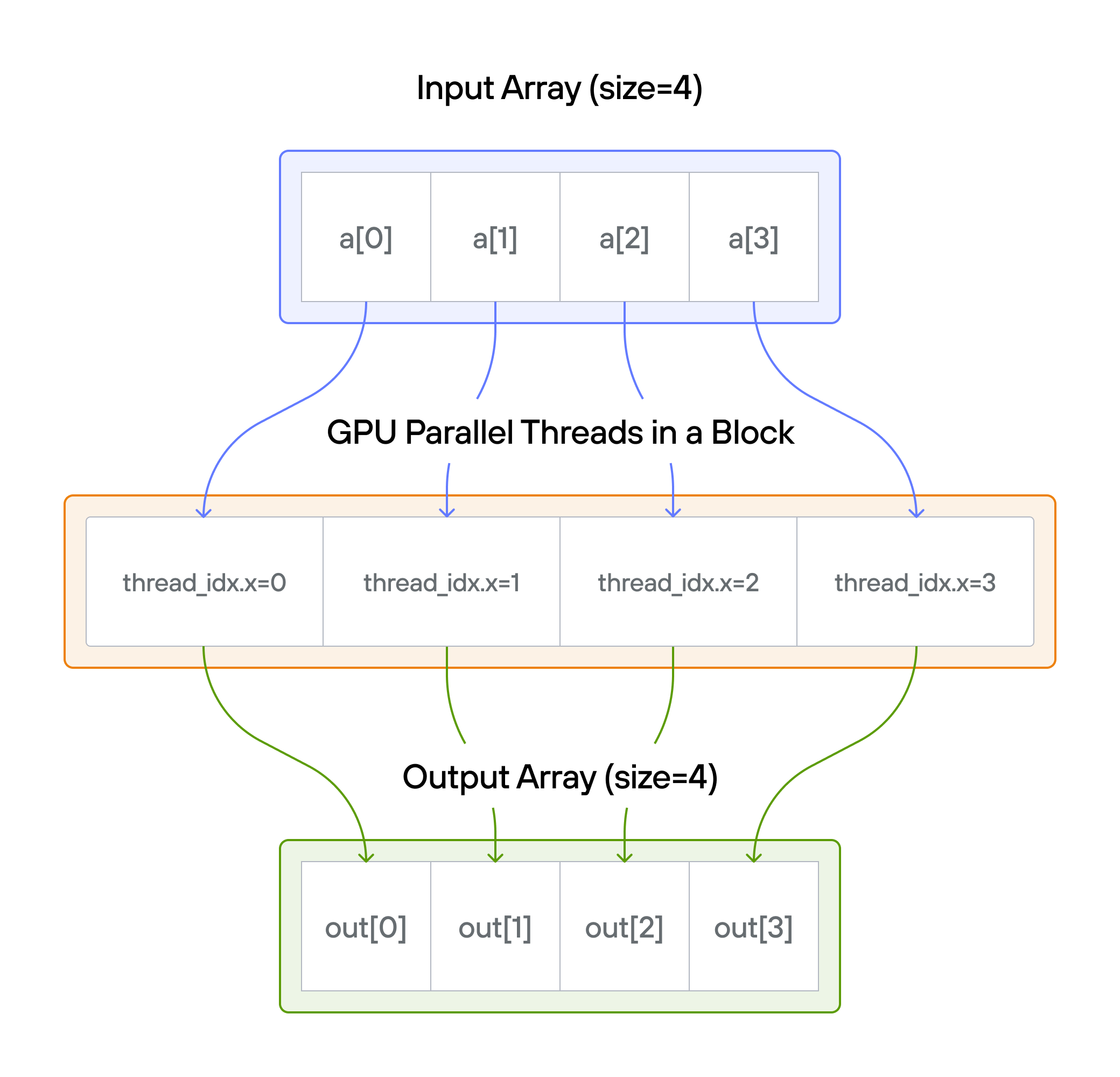
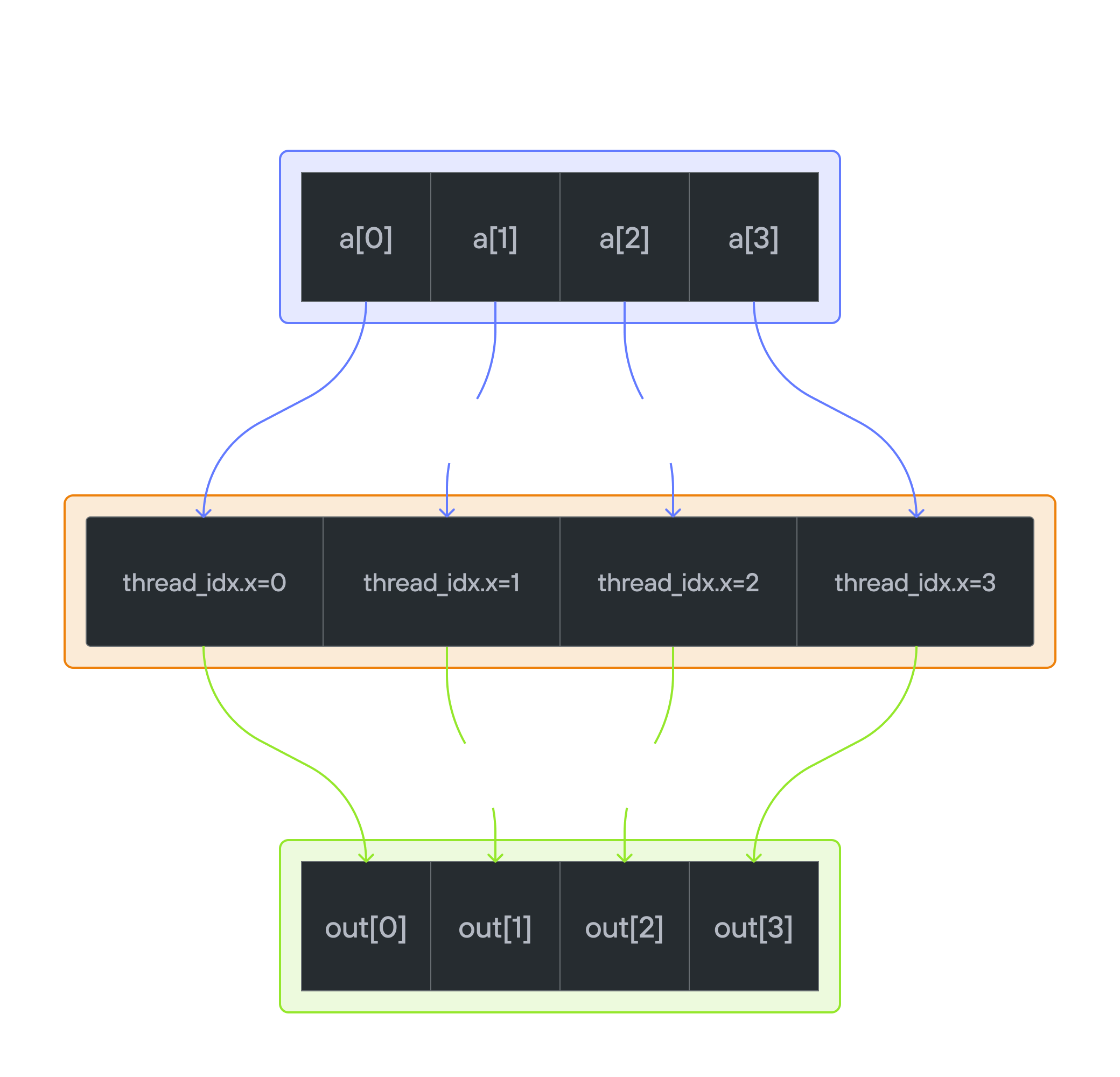
Puzzle 1: Map

Overview

GPU programming is all about parallelism. In this puzzle, each thread will process a single element of the input array independently. Implement a kernel that adds 10 to each position of vector a and stores it in vector output.

Note: You have 1 thread per position.

Key concepts

• Basic GPU kernel structure
• One-to-one thread to data mapping
• Memory access patterns
• Array operations on GPU

For each position \(i\): \[\Large output[i] = a[i] + 10\]

What we cover

🔰 Raw Memory Approach

Start with direct memory manipulation to understand GPU fundamentals.

💡 Preview: Modern Approach with LayoutTensor

See how LayoutTensor simplifies GPU programming with safer, cleaner code.

💡 Tip: Understanding both approaches helps you better appreciate modern GPU programming patterns.

Key concepts

In this puzzle, you’ll learn about:

• Basic GPU kernel structure

• Thread indexing with thread_idx.x

• Simple parallel operations

• Parallelism: Each thread executes independently

• Thread indexing: Access element at position i = thread_idx.x

• Memory access: Read from a[i] and write to output[i]

• Data independence: Each output depends only on its corresponding input

Code to complete

alias SIZE = 4
alias BLOCKS_PER_GRID = 1
alias THREADS_PER_BLOCK = SIZE
alias dtype = DType.float32


fn add_10(
    output: UnsafePointer[Scalar[dtype]], a: UnsafePointer[Scalar[dtype]]
):
    i = thread_idx.x
    # FILL ME IN (roughly 1 line)

View full file: problems/p01/p01.mojo

Running the code

To test your solution, run the following command in your terminal:

uv run poe p01

pixi run p01

Your output will look like this if the puzzle isn’t solved yet:

out: HostBuffer([0.0, 0.0, 0.0, 0.0])
expected: HostBuffer([10.0, 11.0, 12.0, 13.0])

Solution

fn add_10(
    output: UnsafePointer[Scalar[dtype]], a: UnsafePointer[Scalar[dtype]]
):
    i = thread_idx.x
    output[i] = a[i] + 10.0

Why Consider LayoutTensor?

Looking at our traditional implementation above, you might notice some potential issues:

Current approach

i = thread_idx.x
output[i] = a[i] + 10.0

This works for 1D arrays, but what happens when we need to:

• Handle 2D or 3D data?
• Deal with different memory layouts?
• Ensure coalesced memory access?

Preview of future challenges

As we progress through the puzzles, array indexing will become more complex:

# 2D indexing coming in later puzzles
idx = row * WIDTH + col

# 3D indexing
idx = (batch * HEIGHT + row) * WIDTH + col

# With padding
idx = (batch * padded_height + row) * padded_width + col

LayoutTensor preview

LayoutTensor will help us handle these cases more elegantly:

# Future preview - don't worry about this syntax yet!
output[i, j] = a[i, j] + 10.0  # 2D indexing
output[b, i, j] = a[b, i, j] + 10.0  # 3D indexing

We’ll learn about LayoutTensor in detail in Puzzle 4, where these concepts become essential. For now, focus on understanding:

• Basic thread indexing
• Simple memory access patterns
• One-to-one mapping of threads to data

💡 Key Takeaway: While direct indexing works for simple cases, we’ll soon need more sophisticated tools for complex GPU programming patterns.

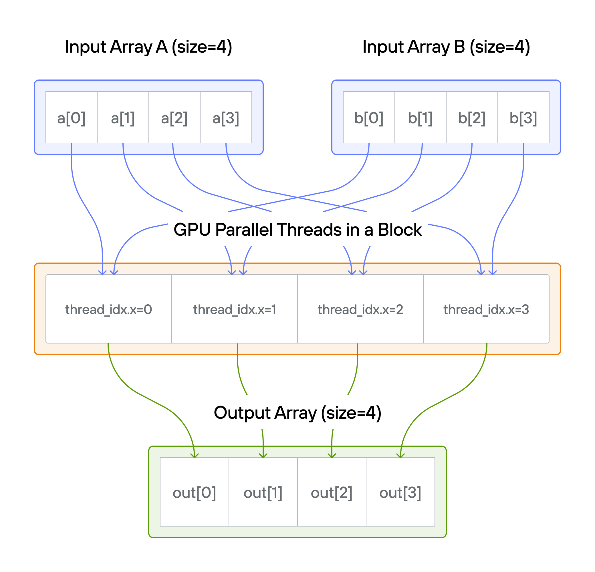
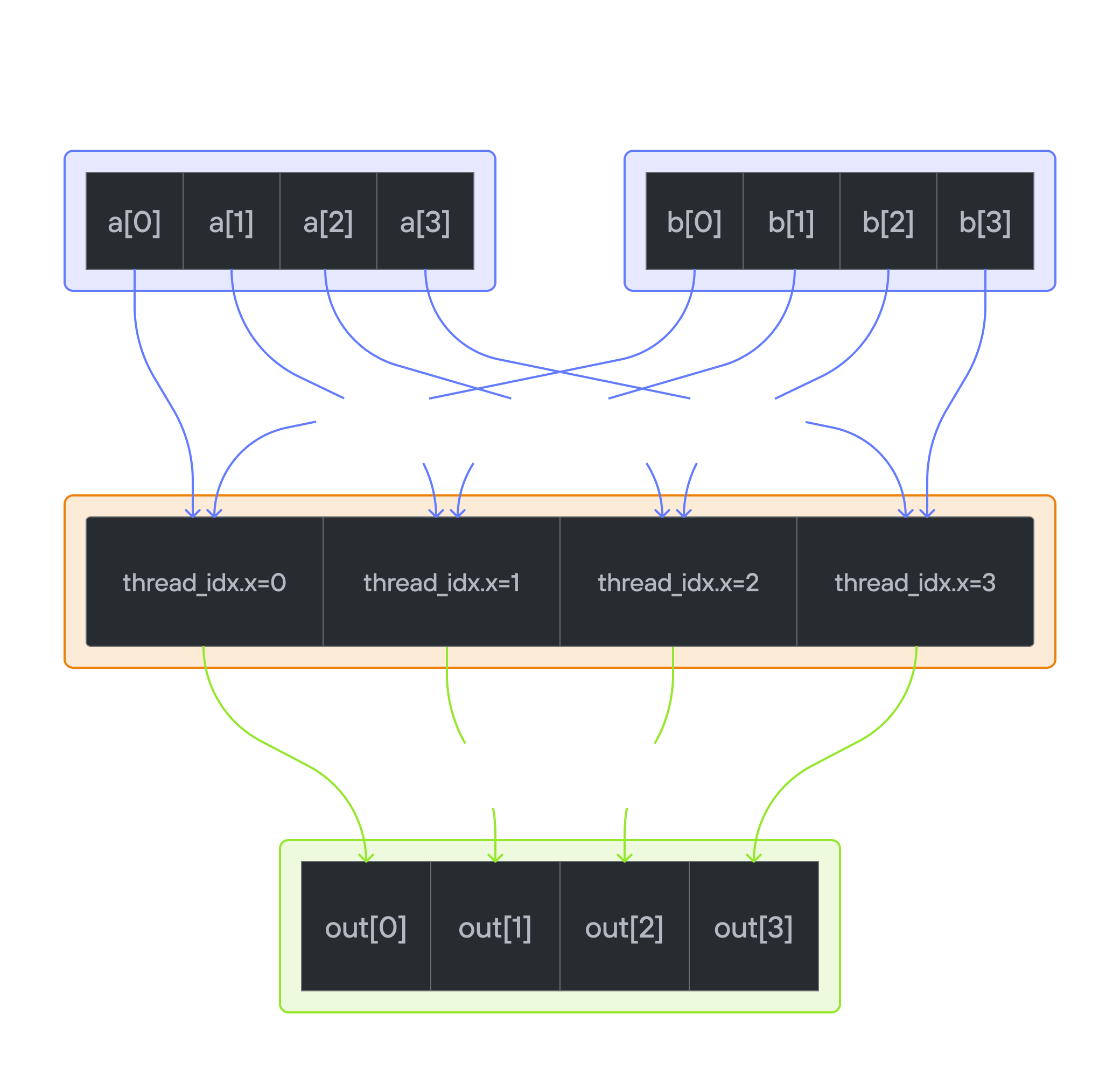
Puzzle 2: Zip

Overview

Implement a kernel that adds together each position of vector a and vector b and stores it in output.

Note: You have 1 thread per position.

Key concepts

In this puzzle, you’ll learn about:

• Processing multiple input arrays in parallel
• Element-wise operations with multiple inputs
• Thread-to-data mapping across arrays
• Memory access patterns with multiple arrays

For each thread \(i\): \[\Large output[i] = a[i] + b[i]\]

Memory access pattern

Thread 0:  a[0] + b[0] → output[0]
Thread 1:  a[1] + b[1] → output[1]
Thread 2:  a[2] + b[2] → output[2]
...

💡 Note: Notice how we’re now managing three arrays (a, b, output) in our kernel. As we progress to more complex operations, managing multiple array accesses will become increasingly challenging.

Code to complete

alias SIZE = 4
alias BLOCKS_PER_GRID = 1
alias THREADS_PER_BLOCK = SIZE
alias dtype = DType.float32


fn add(
    output: UnsafePointer[Scalar[dtype]],
    a: UnsafePointer[Scalar[dtype]],
    b: UnsafePointer[Scalar[dtype]],
):
    i = thread_idx.x
    # FILL ME IN (roughly 1 line)

View full file: problems/p02/p02.mojo

Running the code

To test your solution, run the following command in your terminal:

uv run poe p02

pixi run p02

Your output will look like this if the puzzle isn’t solved yet:

out: HostBuffer([0.0, 0.0, 0.0, 0.0])
expected: HostBuffer([0.0, 2.0, 4.0, 6.0])

Solution

fn add(
    output: UnsafePointer[Scalar[dtype]],
    a: UnsafePointer[Scalar[dtype]],
    b: UnsafePointer[Scalar[dtype]],
):
    i = thread_idx.x
    output[i] = a[i] + b[i]

Looking ahead

While this direct indexing works for simple element-wise operations, consider:

• What if arrays have different layouts?
• What if we need to broadcast one array to another?
• How to ensure coalesced access across multiple arrays?

These questions will be addressed when we introduce LayoutTensor in Puzzle 4.

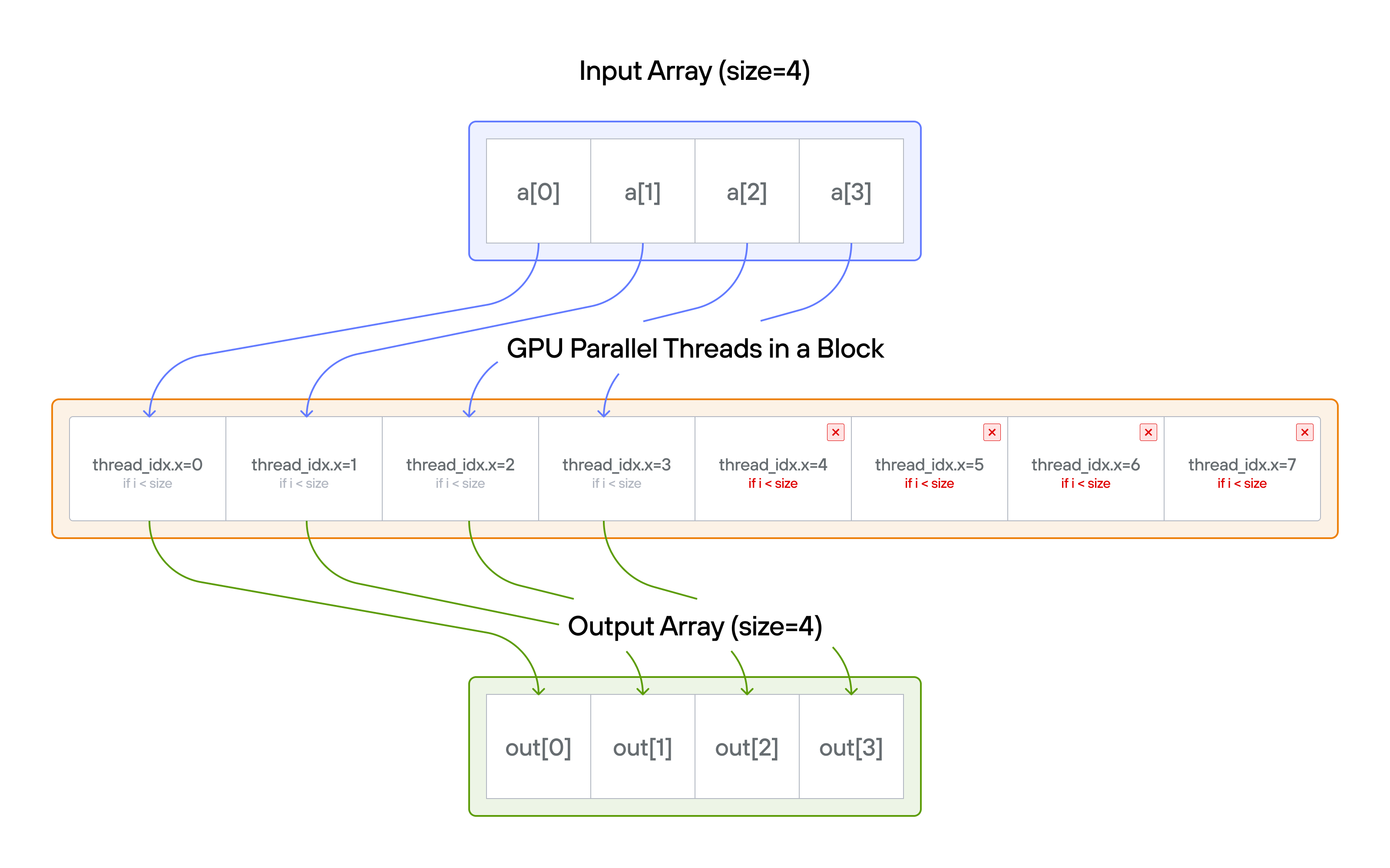
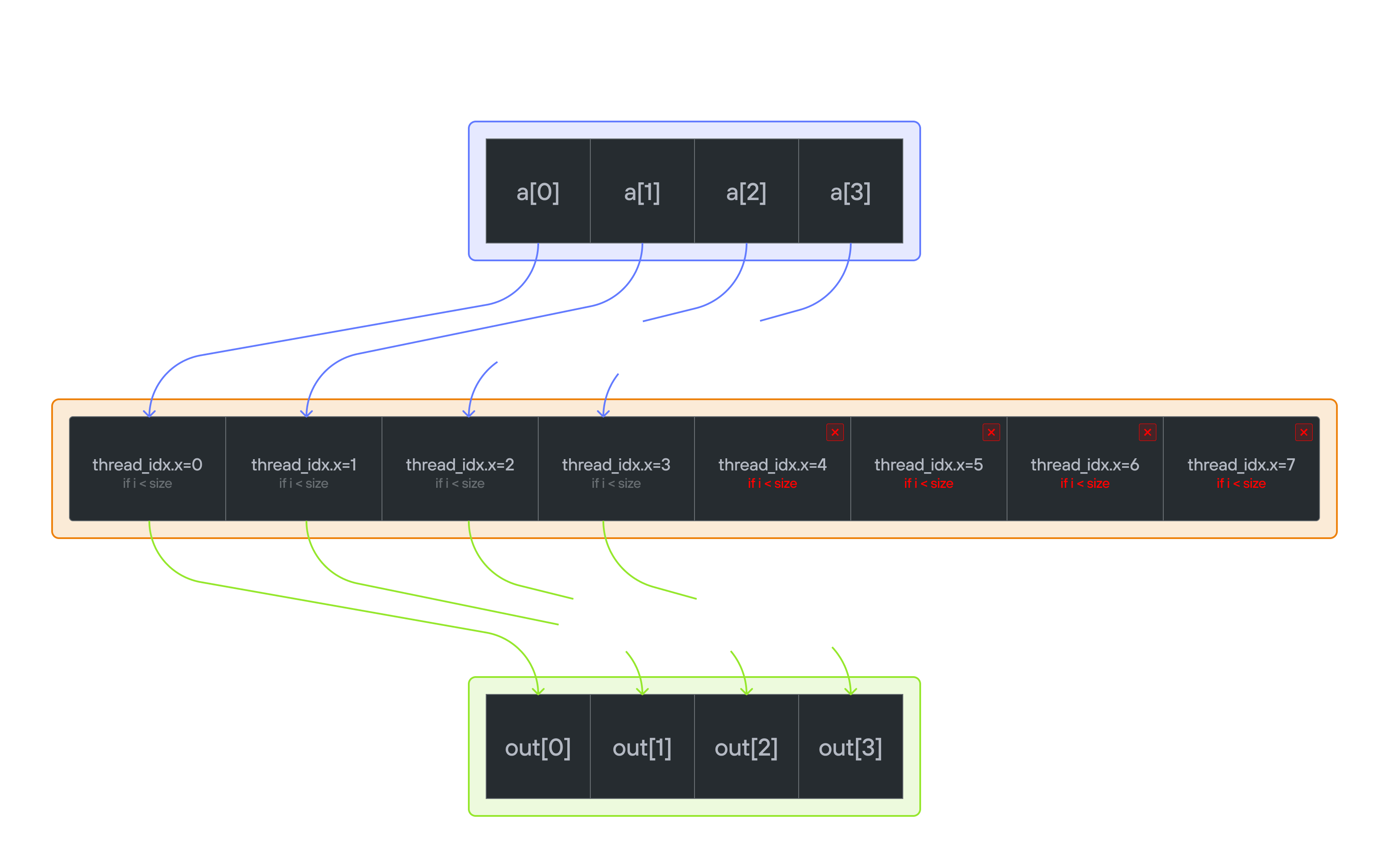
Puzzle 3: Guards

Overview

Implement a kernel that adds 10 to each position of vector a and stores it in vector output.

Note: You have more threads than positions. This means you need to protect against out-of-bounds memory access.

Key concepts

In this puzzle, you’ll learn about:

• Handling thread/data size mismatches
• Preventing out-of-bounds memory access
• Using conditional execution in GPU kernels
• Safe memory access patterns

Mathematical Description

For each thread \(i\): \[\Large \text{if}\ i < \text{size}: output[i] = a[i] + 10\]

Memory Safety Pattern

Thread 0 (i=0):  if 0 < size:  output[0] = a[0] + 10  ✓ Valid
Thread 1 (i=1):  if 1 < size:  output[1] = a[1] + 10  ✓ Valid
Thread 2 (i=2):  if 2 < size:  output[2] = a[2] + 10  ✓ Valid
Thread 3 (i=3):  if 3 < size:  output[3] = a[3] + 10  ✓ Valid
Thread 4 (i=4):  if 4 < size:  ❌ Skip (out of bounds)
Thread 5 (i=5):  if 5 < size:  ❌ Skip (out of bounds)

💡 Note: Boundary checking becomes increasingly complex with:

• Multi-dimensional arrays
• Different array shapes
• Complex access patterns

Code to complete

alias SIZE = 4
alias BLOCKS_PER_GRID = 1
alias THREADS_PER_BLOCK = (8, 1)
alias dtype = DType.float32


fn add_10_guard(
    output: UnsafePointer[Scalar[dtype]],
    a: UnsafePointer[Scalar[dtype]],
    size: Int,
):
    i = thread_idx.x
    # FILL ME IN (roughly 2 lines)

View full file: problems/p03/p03.mojo

Running the code

To test your solution, run the following command in your terminal:

uv run poe p03

pixi run p03

Your output will look like this if the puzzle isn’t solved yet:

out: HostBuffer([0.0, 0.0, 0.0, 0.0])
expected: HostBuffer([10.0, 11.0, 12.0, 13.0])

Solution

fn add_10_guard(
    output: UnsafePointer[Scalar[dtype]],
    a: UnsafePointer[Scalar[dtype]],
    size: Int,
):
    i = thread_idx.x
    if i < size:
        output[i] = a[i] + 10.0

Looking ahead

While simple boundary checks work here, consider these challenges:

• What about 2D/3D array boundaries?
• How to handle different shapes efficiently?
• What if we need padding or edge handling?

Example of growing complexity:

# Current: 1D bounds check
if i < size: ...

# Coming soon: 2D bounds check
if i < height and j < width: ...

# Later: 3D with padding
if i < height and j < width and k < depth and
   i >= padding and j >= padding: ...

These boundary handling patterns will become more elegant when we learn about LayoutTensor in Puzzle 4, which provides built-in shape management.

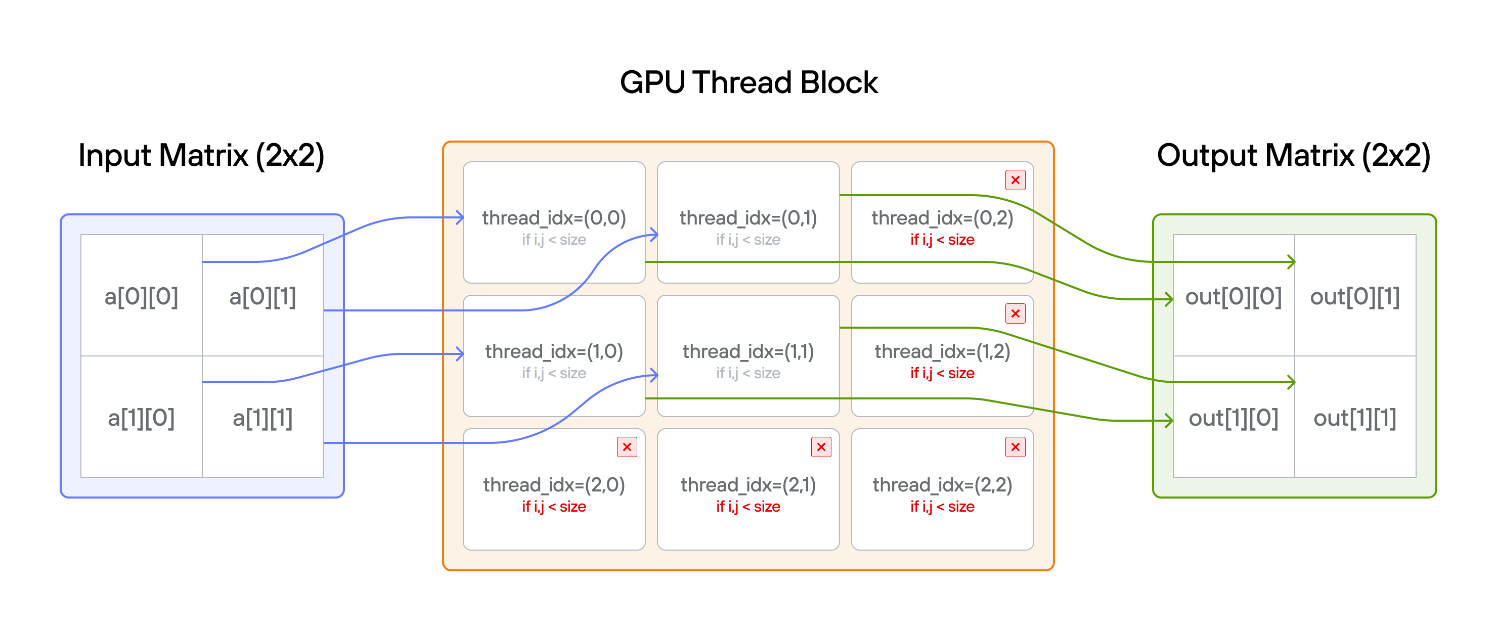
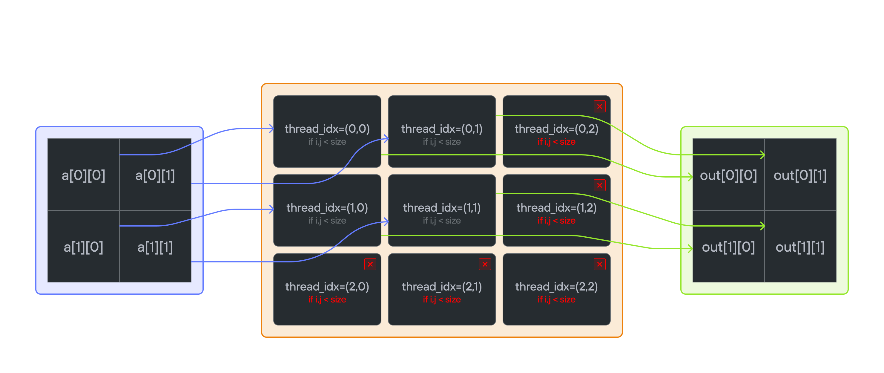
Puzzle 4: 2D Map

Overview

Implement a kernel that adds 10 to each position of 2D square matrix a and stores it in 2D square matrix output.

Note: You have more threads than positions.

Key concepts

• 2D thread indexing
• Matrix operations on GPU
• Handling excess threads
• Memory layout patterns

For each position \((i,j)\): \[\Large output[i,j] = a[i,j] + 10\]

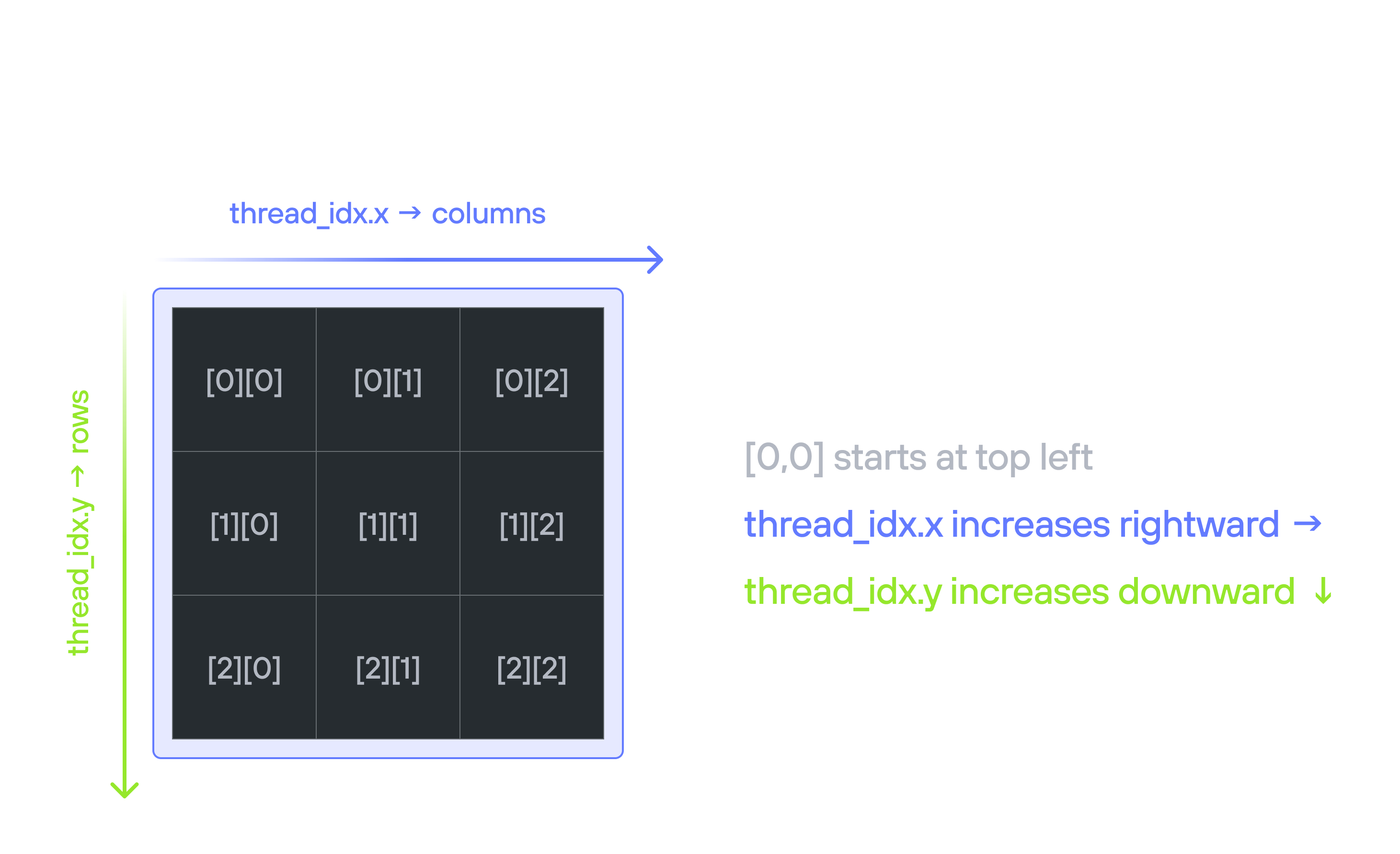
Thread indexing convention

When working with 2D matrices in GPU programming, we follow a natural mapping between thread indices and matrix coordinates:

• thread_idx.y corresponds to the row index
• thread_idx.x corresponds to the column index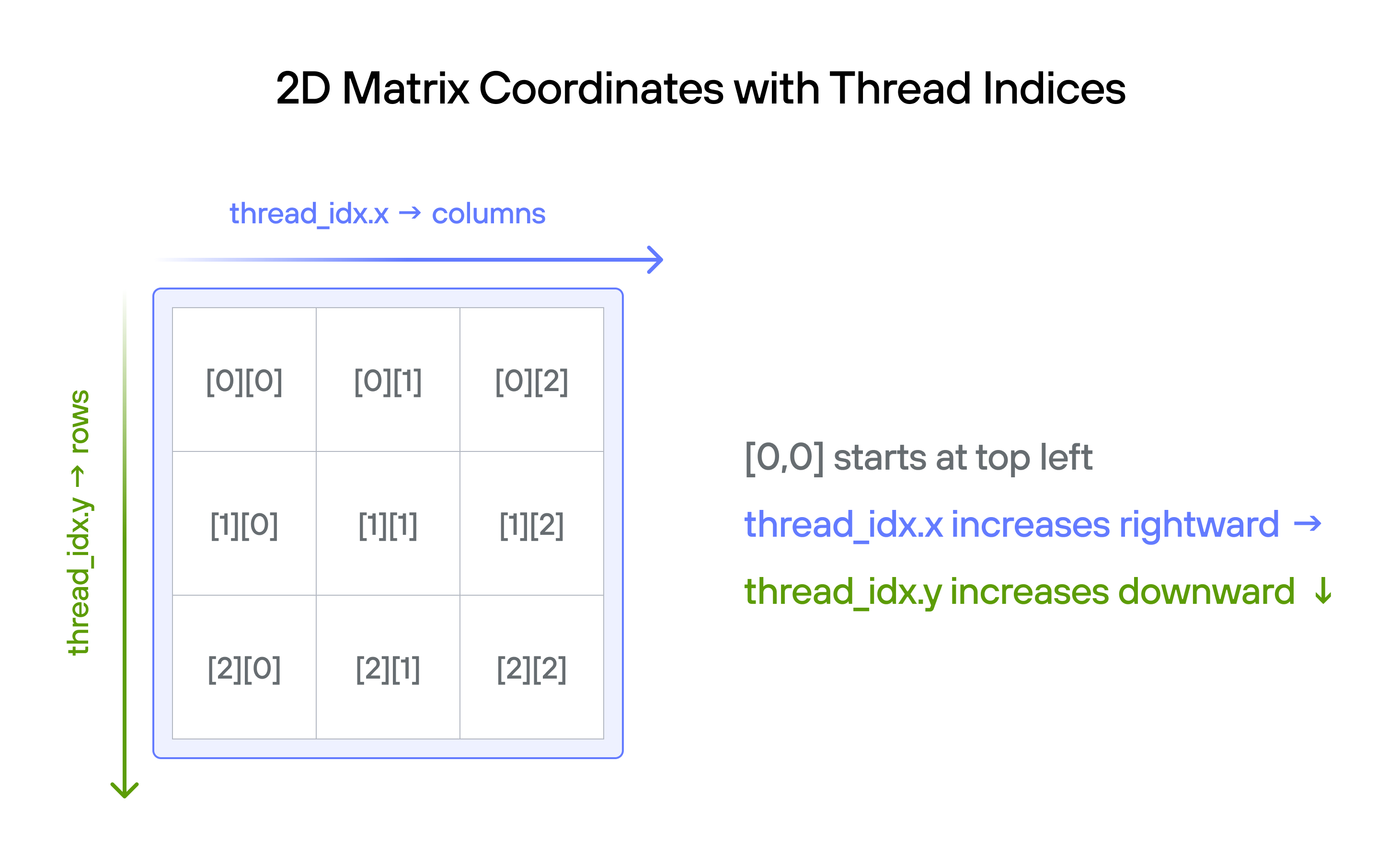

This convention aligns with:

1. The standard mathematical notation where matrix positions are specified as (row, column)
2. The visual representation of matrices where rows go top-to-bottom (y-axis) and columns go left-to-right (x-axis)
3. Common GPU programming patterns where thread blocks are organized in a 2D grid matching the matrix structure

Historical origins

While graphics and image processing typically use \((x,y)\) coordinates, matrix operations in computing have historically used (row, column) indexing. This comes from how early computers stored and processed 2D data: line by line, top to bottom, with each line read left to right. This row-major memory layout proved efficient for both CPUs and GPUs, as it matches how they access memory sequentially. When GPU programming adopted thread blocks for parallel processing, it was natural to map thread_idx.y to rows and thread_idx.x to columns, maintaining consistency with established matrix indexing conventions.

Implementation approaches

🔰 Raw memory approach

Learn how 2D indexing works with manual memory management.

📚 Learn about LayoutTensor

Discover a powerful abstraction that simplifies multi-dimensional array operations and memory management on GPU.

🚀 Modern 2D operations

Put LayoutTensor into practice with natural 2D indexing and automatic bounds checking.

💡 Note: From this puzzle onward, we’ll primarily use LayoutTensor for cleaner, safer GPU code.

Overview

Implement a kernel that adds 10 to each position of 2D square matrix a and stores it in 2D square matrix output.

Note: You have more threads than positions.

Key concepts

In this puzzle, you’ll learn about:

• Working with 2D thread indices (thread_idx.x, thread_idx.y)
• Converting 2D coordinates to 1D memory indices
• Handling boundary checks in two dimensions

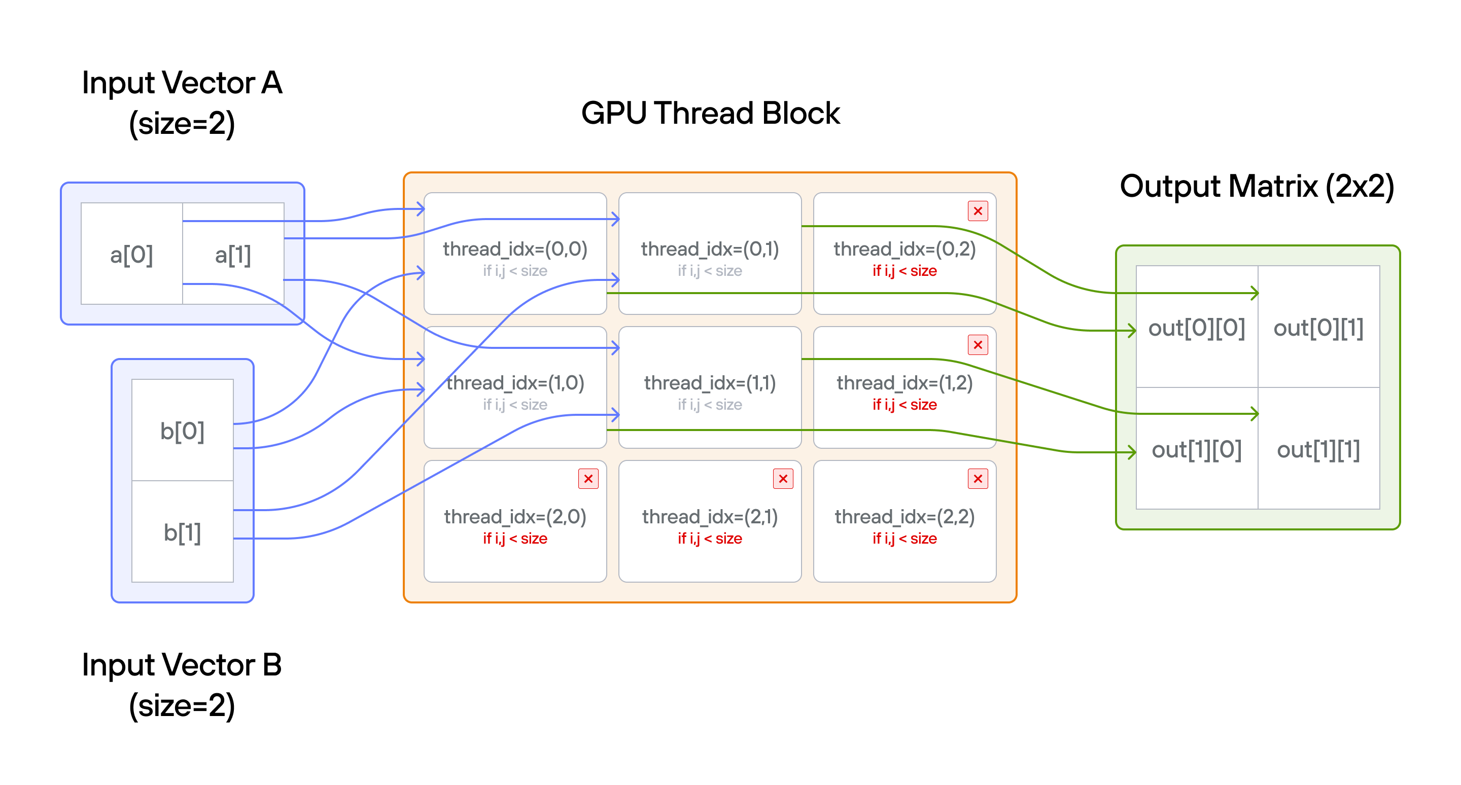
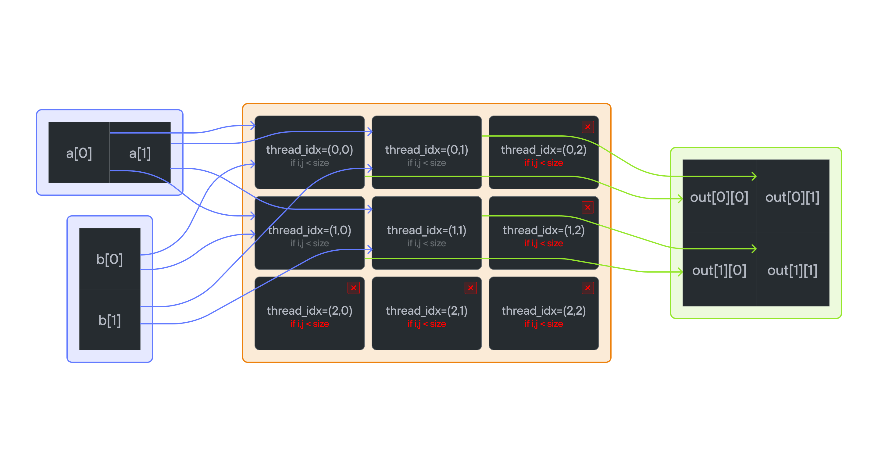
The key insight is understanding how to map from 2D thread coordinates \((i,j)\) to elements in a row-major matrix of size \(n \times n\), while ensuring thread indices are within bounds.

• 2D indexing: Each thread has a unique \((i,j)\) position
• Memory layout: Row-major ordering maps 2D to 1D memory
• Guard condition: Need bounds checking in both dimensions
• Thread bounds: More threads \((3 \times 3)\) than matrix elements \((2 \times 2)\)

Code to complete

alias SIZE = 2
alias BLOCKS_PER_GRID = 1
alias THREADS_PER_BLOCK = (3, 3)
alias dtype = DType.float32


fn add_10_2d(
    output: UnsafePointer[Scalar[dtype]],
    a: UnsafePointer[Scalar[dtype]],
    size: Int,
):
    row = thread_idx.y
    col = thread_idx.x
    # FILL ME IN (roughly 2 lines)

View full file: problems/p04/p04.mojo

Running the code

To test your solution, run the following command in your terminal:

uv run poe p04

pixi run p04

Your output will look like this if the puzzle isn’t solved yet:

out: HostBuffer([0.0, 0.0, 0.0, 0.0])
expected: HostBuffer([10.0, 11.0, 12.0, 13.0])

Solution

fn add_10_2d(
    output: UnsafePointer[Scalar[dtype]],
    a: UnsafePointer[Scalar[dtype]],
    size: Int,
):
    row = thread_idx.y
    col = thread_idx.x
    if row < size and col < size:
        output[row * size + col] = a[row * size + col] + 10.0

Introduction to LayoutTensor

Let’s take a quick break from solving puzzles to preview a powerful abstraction that will make our GPU programming journey more enjoyable: 🥁 … the LayoutTensor.

💡 This is a motivational overview of LayoutTensor’s capabilities. Don’t worry about understanding everything now - we’ll explore each feature in depth as we progress through the puzzles.

The challenge: Growing complexity

Let’s look at the challenges we’ve faced so far:

# Puzzle 1: Simple indexing
output[i] = a[i] + 10.0

# Puzzle 2: Multiple array management
output[i] = a[i] + b[i]

# Puzzle 3: Bounds checking
if i < size:
    output[i] = a[i] + 10.0

As dimensions grow, code becomes more complex:

# Traditional 2D indexing for row-major 2D matrix
idx = row * WIDTH + col
if row < height and col < width:
    output[idx] = a[idx] + 10.0

The solution: A peek at LayoutTensor

LayoutTensor will help us tackle these challenges with elegant solutions. Here’s a glimpse of what’s coming:

1. Natural Indexing: Use tensor[i, j] instead of manual offset calculations
2. Flexible Memory Layouts: Support for row-major, column-major, and tiled organizations
3. Performance Optimization: Efficient memory access patterns for GPU

A taste of what’s ahead

Let’s look at a few examples of what LayoutTensor can do. Don’t worry about understanding all the details now - we’ll cover each feature thoroughly in upcoming puzzles.

Basic usage example

from layout import Layout, LayoutTensor

# Define layout
alias HEIGHT = 2
alias WIDTH = 3
alias layout = Layout.row_major(HEIGHT, WIDTH)

# Create tensor
tensor = LayoutTensor[dtype, layout](buffer.unsafe_ptr())

# Access elements naturally
tensor[0, 0] = 1.0  # First element
tensor[1, 2] = 2.0  # Last element

Preview of advanced features

As we progress through the puzzles, you’ll learn about:

• Shared memory optimizations
• Efficient tiling strategies
• Vectorized operations
• Hardware acceleration
• Optimized memory access patterns

# Column-major layout
layout_col = Layout.col_major(HEIGHT, WIDTH)

# Tiled layout (for better cache utilization)
layout_tiled = tensor.tiled[4, 4](HEIGHT, WIDTH)

Each layout has its advantages:

• Row-major: Elements in a row are contiguous

  # [1 2 3]
  # [4 5 6] -> [1 2 3 4 5 6]
  layout_row = Layout.row_major(2, 3)
  

• Column-major: Elements in a column are contiguous

  # [1 2 3]
  # [4 5 6] -> [1 4 2 5 3 6]
  layout_col = Layout.col_major(2, 3)
  

• Tiled: Elements grouped in tiles for cache efficiency

  # [[1 2] [3 4]] in 2x2 tiles
  layout_tiled = Layout.tiled[2, 2](4, 4)
  

Advanced GPU optimizations

As you progress, you’ll discover LayoutTensor’s powerful features for GPU programming:

1. Memory hierarchy management

# Shared memory allocation
shared_mem = tb[dtype]().row_major[BM, BK]().shared().alloc()

# Register allocation
reg_tile = tb[dtype]().row_major[TM, TN]().local().alloc()

2. Tiling strategies

# Block tiling
block_tile = tensor.tile[BM, BN](block_idx.y, block_idx.x)

# Register tiling
reg_tile = block_tile.tile[TM, TN](thread_row, thread_col)

3. Memory access patterns

# Vectorized access
vec_tensor = tensor.vectorize[1, simd_width]()

# Asynchronous transfers
copy_dram_to_sram_async[thread_layout=layout](dst, src)

4. Hardware acceleration

# Tensor Core operations (coming in later puzzles)
mma_op = TensorCore[dtype, out_type, Index(M, N, K)]()
result = mma_op.mma_op(a_reg, b_reg, c_reg)

💡 Looking ahead: Through these puzzles, you’ll learn to:

• Optimize data access with shared memory
• Implement efficient tiling strategies
• Leverage vectorized operations
• Utilize hardware accelerators
• Master memory access patterns

Each concept builds on the last, gradually taking you from basic tensor operations to advanced GPU programming. Ready to begin? Let’s start with the fundamentals!

Quick example

Let’s put everything together with a simple example that demonstrates the basics of LayoutTensor:

from gpu.host import DeviceContext
from layout import Layout, LayoutTensor

alias HEIGHT = 2
alias WIDTH = 3
alias dtype = DType.float32
alias layout = Layout.row_major(HEIGHT, WIDTH)

fn kernel[dtype: DType, layout: Layout](tensor: LayoutTensor[mut=True, dtype, layout]):
    print("Before:")
    print(tensor)
    tensor[0, 0] += 1
    print("After:")
    print(tensor)

def main():
    ctx = DeviceContext()

    a = ctx.enqueue_create_buffer[dtype](HEIGHT * WIDTH).enqueue_fill(0)
    tensor = LayoutTensor[mut=True, dtype, layout](a.unsafe_ptr())
    # Note: since `tensor` is a device tensor we can't print it without the kernel wrapper
    ctx.enqueue_function[kernel[dtype, layout]](tensor, grid_dim=1, block_dim=1)

    ctx.synchronize()

When we run this code with:

uv run poe layout_tensor_intro

pixi run layout_tensor_intro

Before:
0.0 0.0 0.0
0.0 0.0 0.0
After:
1.0 0.0 0.0
0.0 0.0 0.0

Let’s break down what’s happening:

1. We create a 2 x 3 tensor with row-major layout
2. Initially, all elements are zero
3. Using natural indexing, we modify a single element
4. The change is reflected in our output

This simple example demonstrates key LayoutTensor benefits:

• Clean syntax for tensor creation and access
• Automatic memory layout handling
• Natural multi-dimensional indexing

While this example is straightforward, the same patterns will scale to complex GPU operations in upcoming puzzles. You’ll see how these basic concepts extend to:

• Multi-threaded GPU operations
• Shared memory optimizations
• Complex tiling strategies
• Hardware-accelerated computations

Ready to start your GPU programming journey with LayoutTensor? Let’s dive into the puzzles!

💡 Tip: Keep this example in mind as we progress - we’ll build upon these fundamental concepts to create increasingly sophisticated GPU programs.

LayoutTensor Version

Overview

Implement a kernel that adds 10 to each position of 2D LayoutTensor a and stores it in 2D LayoutTensor output.

Note: You have more threads than positions.

Key concepts

In this puzzle, you’ll learn about:

• Using LayoutTensor for 2D array access
• Direct 2D indexing with tensor[i, j]
• Handling bounds checking with LayoutTensor

The key insight is that LayoutTensor provides a natural 2D indexing interface, abstracting away the underlying memory layout while still requiring bounds checking.

• 2D access: Natural \((i,j)\) indexing with LayoutTensor
• Memory abstraction: No manual row-major calculation needed
• Guard condition: Still need bounds checking in both dimensions
• Thread bounds: More threads \((3 \times 3)\) than tensor elements \((2 \times 2)\)

Code to complete

alias SIZE = 2
alias BLOCKS_PER_GRID = 1
alias THREADS_PER_BLOCK = (3, 3)
alias dtype = DType.float32
alias layout = Layout.row_major(SIZE, SIZE)


fn add_10_2d(
    output: LayoutTensor[mut=True, dtype, layout],
    a: LayoutTensor[mut=True, dtype, layout],
    size: Int,
):
    row = thread_idx.y
    col = thread_idx.x
    # FILL ME IN (roughly 2 lines)

View full file: problems/p04/p04_layout_tensor.mojo

Running the code

To test your solution, run the following command in your terminal:

uv run poe p04_layout_tensor

pixi run p04_layout_tensor

Your output will look like this if the puzzle isn’t solved yet:

out: HostBuffer([0.0, 0.0, 0.0, 0.0])
expected: HostBuffer([10.0, 11.0, 12.0, 13.0])

Solution

fn add_10_2d(
    output: LayoutTensor[mut=True, dtype, layout],
    a: LayoutTensor[mut=True, dtype, layout],
    size: Int,
):
    row = thread_idx.y
    col = thread_idx.x
    if col < size and row < size:
        output[row, col] = a[row, col] + 10.0

Puzzle 5: Broadcast

Overview

Implement a kernel that broadcast adds vector a and vector b and stores it in 2D matrix output.

Note: You have more threads than positions.

Key concepts

• Broadcasting vectors to matrix
• 2D thread management
• Mixed dimension operations
• Memory layout patterns

Implementation approaches

🔰 Raw memory approach

Learn how to handle broadcasting with manual memory indexing.

📐 LayoutTensor Version

Use LayoutTensor to handle mixed-dimension operations.

💡 Note: Notice how LayoutTensor simplifies broadcasting compared to manual indexing.

Overview

Implement a kernel that broadcast adds vector a and vector b and stores it in 2D matrix output.

Note: You have more threads than positions.

Key concepts

In this puzzle, you’ll learn about:

• Broadcasting 1D vectors across different dimensions
• Using 2D thread indices for broadcast operations
• Handling boundary conditions in broadcast patterns

The key insight is understanding how to map elements from two 1D vectors to create a 2D output matrix through broadcasting, while handling thread bounds correctly.

• Broadcasting: Each element of a combines with each element of b
• Thread mapping: 2D thread grid \((3 \times 3)\) for \(2 \times 2\) output
• Vector access: Different access patterns for a and b
• Bounds checking: Guard against threads outside matrix dimensions

Code to complete

alias SIZE = 2
alias BLOCKS_PER_GRID = 1
alias THREADS_PER_BLOCK = (3, 3)
alias dtype = DType.float32


fn broadcast_add(
    output: UnsafePointer[Scalar[dtype]],
    a: UnsafePointer[Scalar[dtype]],
    b: UnsafePointer[Scalar[dtype]],
    size: Int,
):
    row = thread_idx.y
    col = thread_idx.x
    # FILL ME IN (roughly 2 lines)

View full file: problems/p05/p05.mojo

Running the code

To test your solution, run the following command in your terminal:

uv run poe p05

pixi run p05

Your output will look like this if the puzzle isn’t solved yet:

out: HostBuffer([0.0, 0.0, 0.0, 0.0])
expected: HostBuffer([0.0, 1.0, 1.0, 2.0])

Solution

fn broadcast_add(
    output: UnsafePointer[Scalar[dtype]],
    a: UnsafePointer[Scalar[dtype]],
    b: UnsafePointer[Scalar[dtype]],
    size: Int,
):
    row = thread_idx.y
    col = thread_idx.x
    if row < size and col < size:
        output[row * size + col] = a[col] + b[row]

LayoutTensor Version

Overview

Implement a kernel that broadcast adds 1D LayoutTensor a and 1D LayoutTensor b and stores it in 2D LayoutTensor output.

Note: You have more threads than positions.

Key concepts

In this puzzle, you’ll learn about:

• Using LayoutTensor for broadcast operations
• Working with different tensor shapes
• Handling 2D indexing with LayoutTensor

The key insight is that LayoutTensor allows natural broadcasting through different tensor shapes: \((1, n)\) and \((n, 1)\) to \((n,n)\), while still requiring bounds checking.

• Tensor shapes: Input vectors have shapes \((1, n)\) and \((n, 1)\)
• Broadcasting: Output combines both dimensions to \((n,n)\)
• Guard condition: Still need bounds checking for output size
• Thread bounds: More threads \((3 \times 3)\) than tensor elements \((2 \times 2)\)

Code to complete

alias SIZE = 2
alias BLOCKS_PER_GRID = 1
alias THREADS_PER_BLOCK = (3, 3)
alias dtype = DType.float32
alias out_layout = Layout.row_major(SIZE, SIZE)
alias a_layout = Layout.row_major(1, SIZE)
alias b_layout = Layout.row_major(SIZE, 1)


fn broadcast_add[
    out_layout: Layout,
    a_layout: Layout,
    b_layout: Layout,
](
    output: LayoutTensor[mut=True, dtype, out_layout],
    a: LayoutTensor[mut=False, dtype, a_layout],
    b: LayoutTensor[mut=False, dtype, b_layout],
    size: Int,
):
    row = thread_idx.y
    col = thread_idx.x
    # FILL ME IN (roughly 2 lines)

View full file: problems/p05/p05_layout_tensor.mojo

Running the code

To test your solution, run the following command in your terminal:

uv run poe p05_layout_tensor

pixi run p05_layout_tensor

Your output will look like this if the puzzle isn’t solved yet:

out: HostBuffer([0.0, 0.0, 0.0, 0.0])
expected: HostBuffer([0.0, 1.0, 1.0, 2.0])

Solution

fn broadcast_add[
    out_layout: Layout,
    a_layout: Layout,
    b_layout: Layout,
](
    output: LayoutTensor[mut=True, dtype, out_layout],
    a: LayoutTensor[mut=False, dtype, a_layout],
    b: LayoutTensor[mut=False, dtype, b_layout],
    size: Int,
):
    row = thread_idx.y
    col = thread_idx.x
    if row < size and col < size:
        output[row, col] = a[0, col] + b[row, 0]

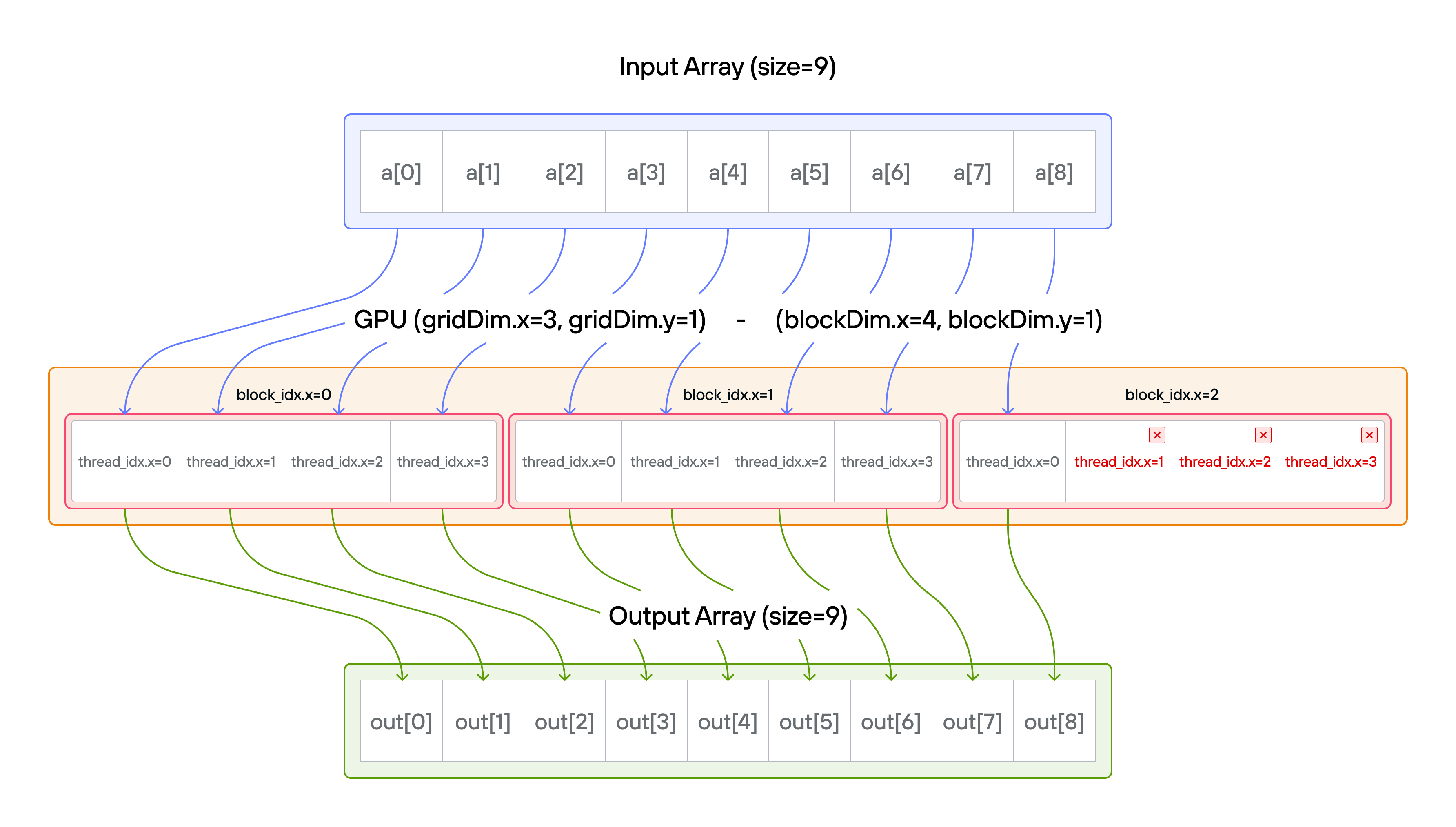
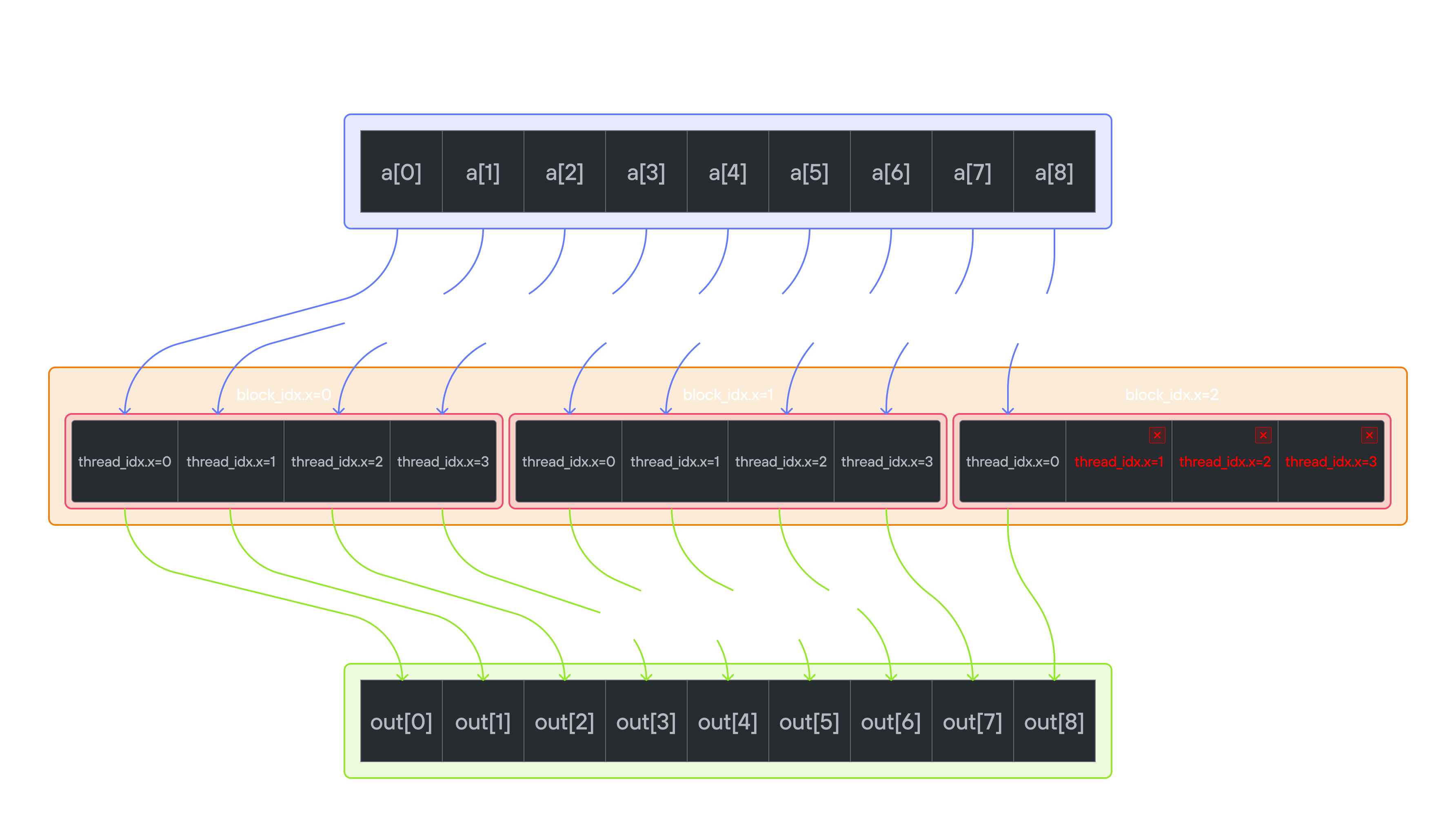
Puzzle 6: Blocks

Overview

Implement a kernel that adds 10 to each position of vector a and stores it in output.

Note: You have fewer threads per block than the size of a.

Key concepts

In this puzzle, you’ll learn about:

• Processing data larger than thread block size
• Coordinating multiple blocks of threads
• Computing global thread positions

The key insight is understanding how blocks of threads work together to process data that’s larger than a single block’s capacity, while maintaining correct element-to-thread mapping.

Code to complete

alias SIZE = 9
alias BLOCKS_PER_GRID = (3, 1)
alias THREADS_PER_BLOCK = (4, 1)
alias dtype = DType.float32


fn add_10_blocks(
    output: UnsafePointer[Scalar[dtype]],
    a: UnsafePointer[Scalar[dtype]],
    size: Int,
):
    i = block_dim.x * block_idx.x + thread_idx.x
    # FILL ME IN (roughly 2 lines)

View full file: problems/p06/p06.mojo

Running the code

To test your solution, run the following command in your terminal:

uv run poe p06

pixi run p06

Your output will look like this if the puzzle isn’t solved yet:

out: HostBuffer([0.0, 0.0, 0.0, 0.0, 0.0, 0.0, 0.0, 0.0, 0.0])
expected: HostBuffer([10.0, 11.0, 12.0, 13.0, 14.0, 15.0, 16.0, 17.0, 18.0])

Solution

fn add_10_blocks(
    output: UnsafePointer[Scalar[dtype]],
    a: UnsafePointer[Scalar[dtype]],
    size: Int,
):
    i = block_dim.x * block_idx.x + thread_idx.x
    if i < size:
        output[i] = a[i] + 10.0

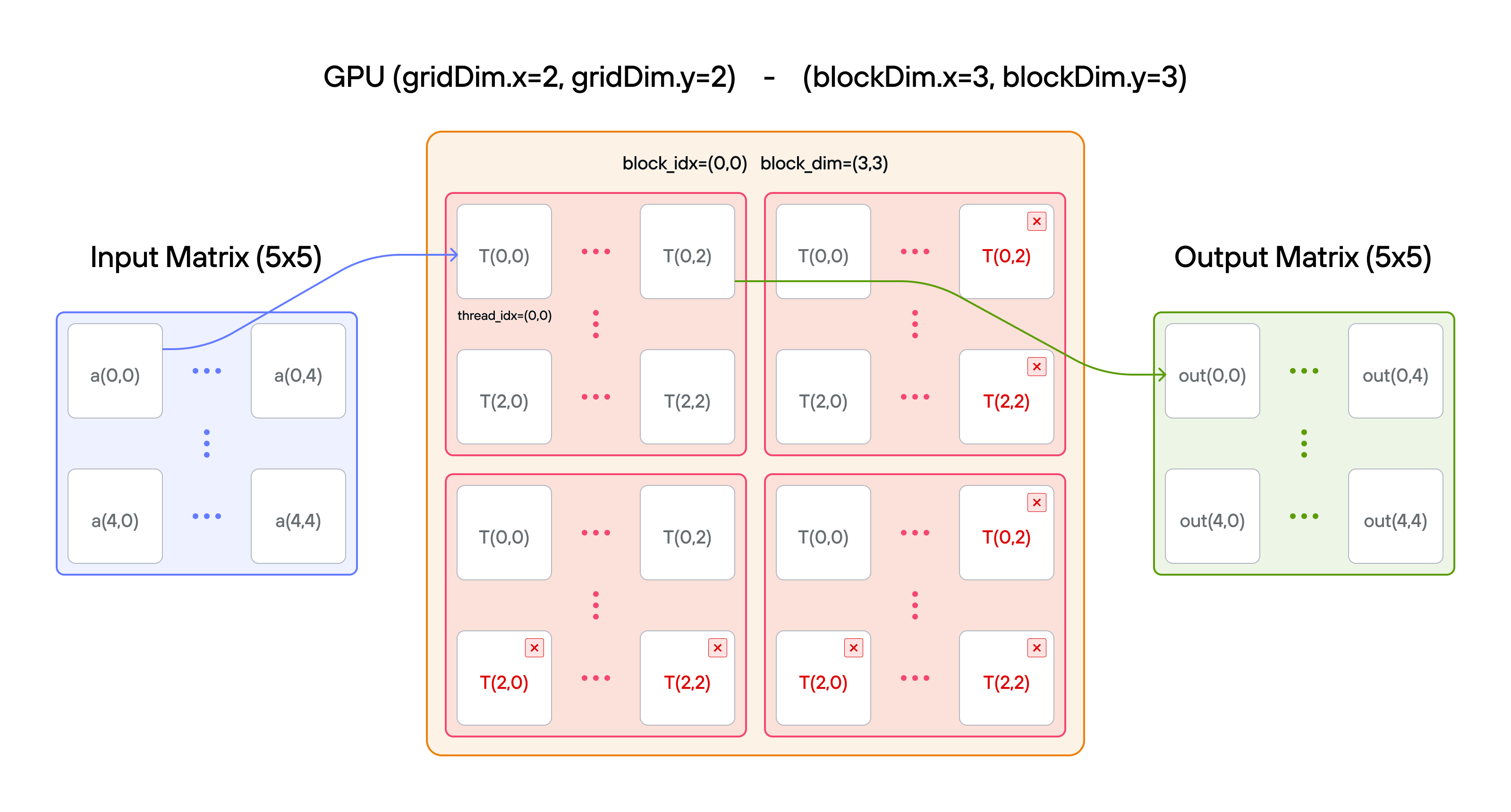
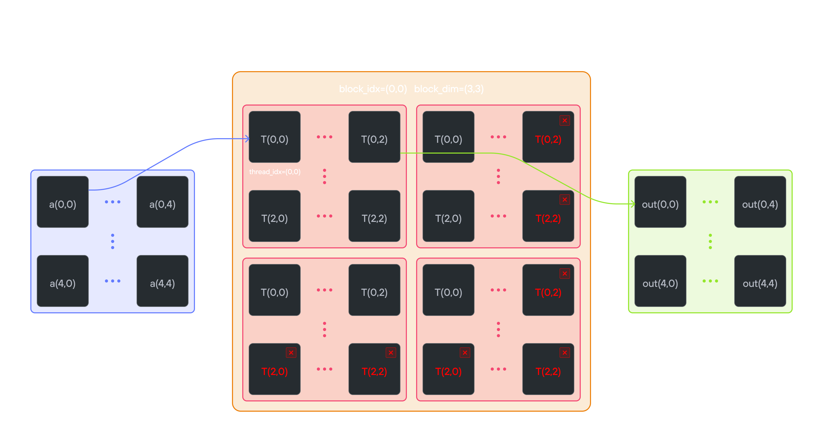
Puzzle 7: 2D Blocks

Overview

Implement a kernel that adds 10 to each position of matrix a and stores it in output.

Note: You have fewer threads per block than the size of a in both directions.

Key concepts

• Block-based processing
• Grid-block coordination
• Multi-block indexing
• Memory access patterns

🔑 2D thread indexing convention

We extend the block-based indexing from puzzle 4 to 2D:

Global position calculation:
row = block_dim.y * block_idx.y + thread_idx.y
col = block_dim.x * block_idx.x + thread_idx.x

For example, with 2×2 blocks in a 4×4 grid:

Block (0,0):   Block (1,0):
[0,0  0,1]     [0,2  0,3]
[1,0  1,1]     [1,2  1,3]

Block (0,1):   Block (1,1):
[2,0  2,1]     [2,2  2,3]
[3,0  3,1]     [3,2  3,3]

Each position shows (row, col) for that thread’s global index. The block dimensions and indices work together to ensure:

• Continuous coverage of the 2D space
• No overlap between blocks
• Efficient memory access patterns

Implementation approaches

🔰 Raw memory approach

Learn how to handle multi-block operations with manual indexing.

📐 LayoutTensor Version

Use LayoutTensor features to elegantly handle block-based processing.

💡 Note: See how LayoutTensor simplifies block coordination and memory access patterns.

Overview

Implement a kernel that adds 10 to each position of matrix a and stores it in output.

Note: You have fewer threads per block than the size of a in both directions.

Key concepts

In this puzzle, you’ll learn about:

• Working with 2D block and thread arrangements
• Handling matrix data larger than block size
• Converting between 2D and linear memory access

The key insight is understanding how to coordinate multiple blocks of threads to process a 2D matrix that’s larger than a single block’s dimensions.

Configuration

• Matrix size: \(5 \times 5\) elements
• 2D blocks: Each block processes a \(3 \times 3\) region
• Grid layout: Blocks arranged in \(2 \times 2\) grid
• Total threads: \(36\) for \(25\) elements
• Memory pattern: Row-major storage for 2D data
• Coverage: Ensuring all matrix elements are processed

Code to complete

alias SIZE = 5
alias BLOCKS_PER_GRID = (2, 2)
alias THREADS_PER_BLOCK = (3, 3)
alias dtype = DType.float32


fn add_10_blocks_2d(
    output: UnsafePointer[Scalar[dtype]],
    a: UnsafePointer[Scalar[dtype]],
    size: Int,
):
    row = block_dim.y * block_idx.y + thread_idx.y
    col = block_dim.x * block_idx.x + thread_idx.x
    # FILL ME IN (roughly 2 lines)

View full file: problems/p07/p07.mojo

Running the code

To test your solution, run the following command in your terminal:

uv run poe p07

pixi run p07

Your output will look like this if the puzzle isn’t solved yet:

out: HostBuffer([0.0, 0.0, 0.0, ... , 0.0])
expected: HostBuffer([11.0, 11.0, 11.0, ... , 11.0])

Solution

fn add_10_blocks_2d(
    output: UnsafePointer[Scalar[dtype]],
    a: UnsafePointer[Scalar[dtype]],
    size: Int,
):
    row = block_dim.y * block_idx.y + thread_idx.y
    col = block_dim.x * block_idx.x + thread_idx.x
    if row < size and col < size:
        output[row * size + col] = a[row * size + col] + 10.0

LayoutTensor Version

Overview

Implement a kernel that adds 10 to each position of 2D LayoutTensor a and stores it in 2D LayoutTensor output.

Note: You have fewer threads per block than the size of a in both directions.

Key concepts

In this puzzle, you’ll learn about:

• Using LayoutTensor with multiple blocks
• Handling large matrices with 2D block organization
• Combining block indexing with LayoutTensor access

The key insight is that LayoutTensor simplifies 2D indexing while still requiring proper block coordination for large matrices.

Configuration

• Matrix size: \(5 \times 5\) elements
• Layout handling: LayoutTensor manages row-major organization
• Block coordination: Multiple blocks cover the full matrix
• 2D indexing: Natural \((i,j)\) access with bounds checking
• Total threads: \(36\) for \(25\) elements
• Thread mapping: Each thread processes one matrix element

Code to complete

alias SIZE = 5
alias BLOCKS_PER_GRID = (2, 2)
alias THREADS_PER_BLOCK = (3, 3)
alias dtype = DType.float32
alias out_layout = Layout.row_major(SIZE, SIZE)
alias a_layout = Layout.row_major(SIZE, SIZE)


fn add_10_blocks_2d[
    out_layout: Layout,
    a_layout: Layout,
](
    output: LayoutTensor[mut=True, dtype, out_layout],
    a: LayoutTensor[mut=False, dtype, a_layout],
    size: Int,
):
    row = block_dim.y * block_idx.y + thread_idx.y
    col = block_dim.x * block_idx.x + thread_idx.x
    # FILL ME IN (roughly 2 lines)

View full file: problems/p07/p07_layout_tensor.mojo

Running the code

To test your solution, run the following command in your terminal:

uv run poe p07_layout_tensor

pixi run p07_layout_tensor

Your output will look like this if the puzzle isn’t solved yet:

out: HostBuffer([0.0, 0.0, 0.0, ... , 0.0])
expected: HostBuffer([11.0, 11.0, 11.0, ... , 11.0])

Solution

fn add_10_blocks_2d[
    out_layout: Layout,
    a_layout: Layout,
](
    output: LayoutTensor[mut=True, dtype, out_layout],
    a: LayoutTensor[mut=False, dtype, a_layout],
    size: Int,
):
    row = block_dim.y * block_idx.y + thread_idx.y
    col = block_dim.x * block_idx.x + thread_idx.x
    if row < size and col < size:
        output[row, col] = a[row, col] + 10.0

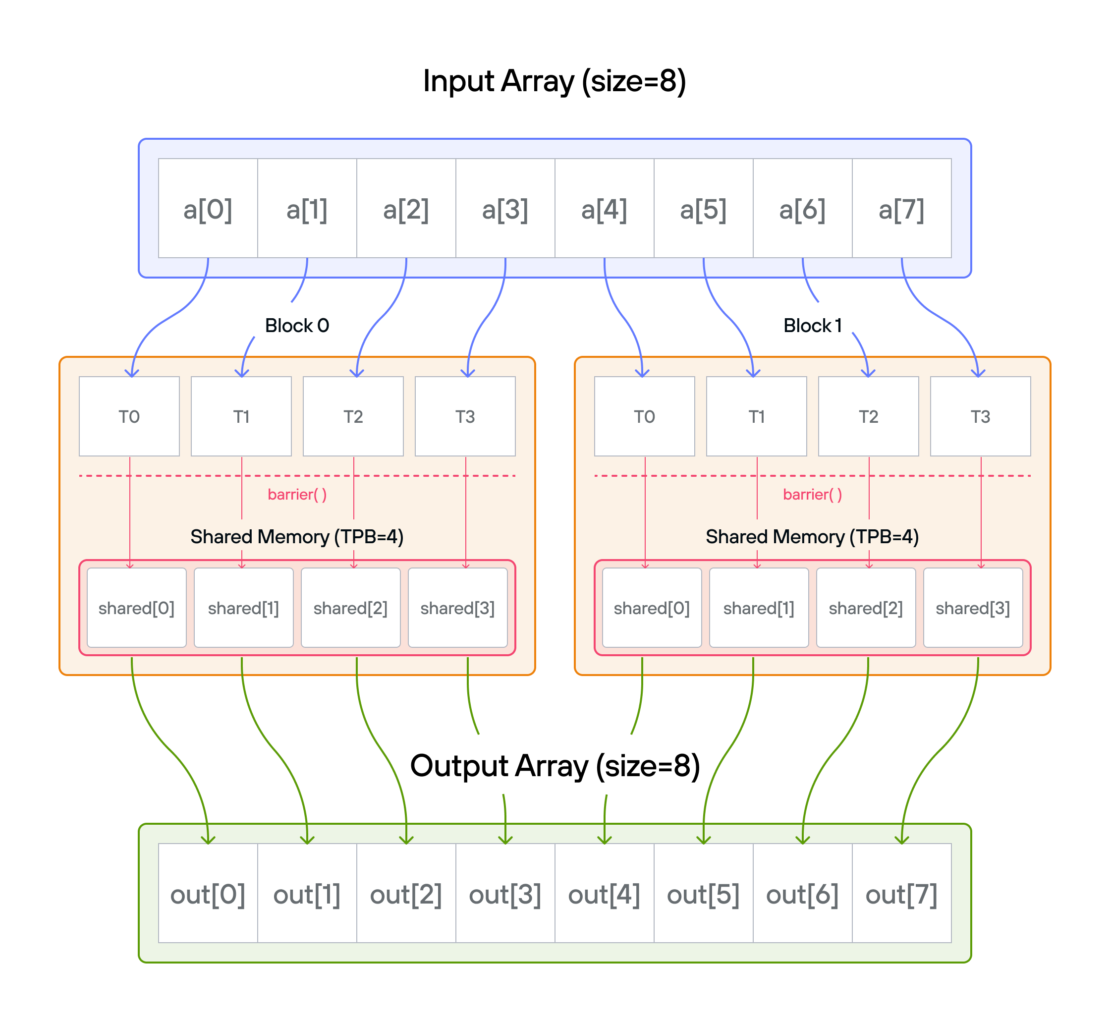
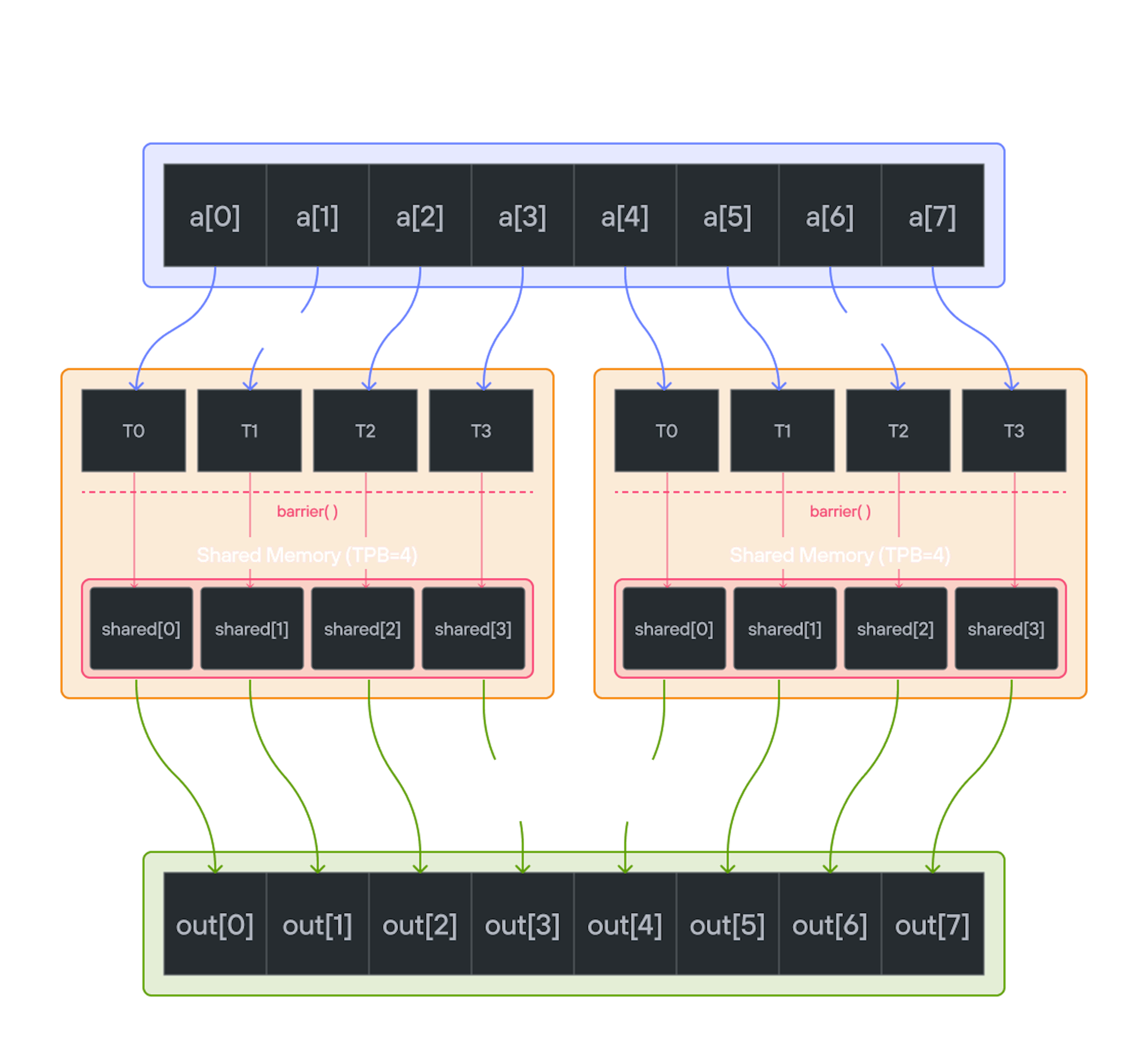
Puzzle 8: Shared Memory

Overview

Implement a kernel that adds 10 to each position of a vector a and stores it in vector output.

Note: You have fewer threads per block than the size of a.

Implementation approaches

🔰 Raw memory approach

Learn how to manually manage shared memory and synchronization.

📐 LayoutTensor Version

Use LayoutTensor’s built-in shared memory management features.

💡 Note: Experience how LayoutTensor simplifies shared memory operations while maintaining performance.

Overview

Implement a kernel that adds 10 to each position of a vector a and stores it in output.

Note: You have fewer threads per block than the size of a.

Key concepts

In this puzzle, you’ll learn about:

• Using shared memory within thread blocks
• Synchronizing threads with barriers
• Managing block-local data storage

The key insight is understanding how shared memory provides fast, block-local storage that all threads in a block can access, requiring careful coordination between threads.

Configuration

• Array size: SIZE = 8 elements
• Threads per block: TPB = 4
• Number of blocks: 2
• Shared memory: TPB elements per block

Notes:

• Shared memory: Fast storage shared by threads in a block
• Thread sync: Coordination using barrier()
• Memory scope: Shared memory only visible within block
• Access pattern: Local vs global indexing

Warning: Each block can only have a constant amount of shared memory that threads in that block can read and write to. This needs to be a literal python constant, not a variable. After writing to shared memory you need to call barrier to ensure that threads do not cross.

Educational Note: In this specific puzzle, the barrier() isn’t strictly necessary since each thread only accesses its own shared memory location. However, it’s included to teach proper shared memory synchronization patterns for more complex scenarios where threads need to coordinate access to shared data.

Code to complete

alias TPB = 4
alias SIZE = 8
alias BLOCKS_PER_GRID = (2, 1)
alias THREADS_PER_BLOCK = (TPB, 1)
alias dtype = DType.float32


fn add_10_shared(
    output: UnsafePointer[Scalar[dtype]],
    a: UnsafePointer[Scalar[dtype]],
    size: Int,
):
    shared = stack_allocation[
        TPB,
        Scalar[dtype],
        address_space = AddressSpace.SHARED,
    ]()
    global_i = block_dim.x * block_idx.x + thread_idx.x
    local_i = thread_idx.x
    # local data into shared memory
    if global_i < size:
        shared[local_i] = a[global_i]

    # wait for all threads to complete
    # works within a thread block
    barrier()

    # FILL ME IN (roughly 2 lines)

View full file: problems/p08/p08.mojo

Running the code

To test your solution, run the following command in your terminal:

uv run poe p08

pixi run p08

Your output will look like this if the puzzle isn’t solved yet:

out: HostBuffer([0.0, 0.0, 0.0, 0.0, 0.0, 0.0, 0.0, 0.0])
expected: HostBuffer([11.0, 11.0, 11.0, 11.0, 11.0, 11.0, 11.0, 11.0])

Solution

fn add_10_shared(
    output: UnsafePointer[Scalar[dtype]],
    a: UnsafePointer[Scalar[dtype]],
    size: Int,
):
    shared = stack_allocation[
        TPB,
        Scalar[dtype],
        address_space = AddressSpace.SHARED,
    ]()
    global_i = block_dim.x * block_idx.x + thread_idx.x
    local_i = thread_idx.x
    # local data into shared memory
    if global_i < size:
        shared[local_i] = a[global_i]

    # wait for all threads to complete
    # works within a thread block
    # Note: barrier is not strictly needed here since each thread only accesses its own shared memory location.
    # However, it's included to teach proper shared memory synchronization patterns
    # for more complex scenarios where threads need to coordinate access to shared data.
    # For this specific puzzle, we can remove the barrier since each thread only accesses its own shared memory location.
    barrier()

    # process using shared memory
    if global_i < size:
        output[global_i] = shared[local_i] + 10

Overview

Implement a kernel that adds 10 to each position of a 1D ayoutTensor a and stores it in 1D LayoutTensor output.

Note: You have fewer threads per block than the size of a.

Key concepts

In this puzzle, you’ll learn about:

• Using LayoutTensor’s shared memory features
• Thread synchronization with shared memory
• Block-local data management with tensor builder

The key insight is how LayoutTensor simplifies shared memory management while maintaining the performance benefits of block-local storage.

Configuration

• Array size: SIZE = 8 elements
• Threads per block: TPB = 4
• Number of blocks: 2
• Shared memory: TPB elements per block

Key differences from raw approach

1. Memory allocation: We will use LayoutTensorBuild instead of stack_allocation

   # Raw approach
   shared = stack_allocation[TPB, Scalar[dtype]]()
   
   # LayoutTensor approach
   shared = LayoutTensorBuild[dtype]().row_major[TPB]().shared().alloc()
   

2. Memory access: Same syntax

   # Raw approach
   shared[local_i] = a[global_i]
   
   # LayoutTensor approach
   shared[local_i] = a[global_i]
   

3. Safety features:

   • Type safety
   • Layout management
   • Memory alignment handling

Note: LayoutTensor handles memory layout, but you still need to manage thread synchronization with barrier() when using shared memory.

Educational Note: In this specific puzzle, the barrier() isn’t strictly necessary since each thread only accesses its own shared memory location. However, it’s included to teach proper shared memory synchronization patterns for more complex scenarios where threads need to coordinate access to shared data.

Code to complete

alias TPB = 4
alias SIZE = 8
alias BLOCKS_PER_GRID = (2, 1)
alias THREADS_PER_BLOCK = (TPB, 1)
alias dtype = DType.float32
alias layout = Layout.row_major(SIZE)


fn add_10_shared_layout_tensor[
    layout: Layout
](
    output: LayoutTensor[mut=True, dtype, layout],
    a: LayoutTensor[mut=True, dtype, layout],
    size: Int,
):
    # Allocate shared memory using tensor builder
    shared = tb[dtype]().row_major[TPB]().shared().alloc()

    global_i = block_dim.x * block_idx.x + thread_idx.x
    local_i = thread_idx.x

    if global_i < size:
        shared[local_i] = a[global_i]

    barrier()

    # FILL ME IN (roughly 2 lines)

View full file: problems/p08/p08_layout_tensor.mojo

Running the code

To test your solution, run the following command in your terminal:

uv run poe p08_layout_tensor

pixi run p08_layout_tensor

Your output will look like this if the puzzle isn’t solved yet:

out: HostBuffer([0.0, 0.0, 0.0, 0.0, 0.0, 0.0, 0.0, 0.0])
expected: HostBuffer([11.0, 11.0, 11.0, 11.0, 11.0, 11.0, 11.0, 11.0])

Solution

fn add_10_shared_layout_tensor[
    layout: Layout
](
    output: LayoutTensor[mut=True, dtype, layout],
    a: LayoutTensor[mut=True, dtype, layout],
    size: Int,
):
    # Allocate shared memory using tensor builder
    shared = tb[dtype]().row_major[TPB]().shared().alloc()

    global_i = block_dim.x * block_idx.x + thread_idx.x
    local_i = thread_idx.x

    if global_i < size:
        shared[local_i] = a[global_i]

    # Note: barrier is not strictly needed here since each thread only accesses its own shared memory location.
    # However, it's included to teach proper shared memory synchronization patterns
    # for more complex scenarios where threads need to coordinate access to shared data.
    # For this specific puzzle, we can remove the barrier since each thread only accesses its own shared memory location.
    barrier()

    if global_i < size:
        output[global_i] = shared[local_i] + 10

Puzzle 9: GPU Debugging Workflow

The moment every GPU programmer faces

You’ve learned to write GPU kernels, work with shared memory, and coordinate thousands of parallel threads. Your code compiles perfectly. You run it with confidence, expecting beautiful results, and then…

• CRASH
• Wrong results
• Infinite hang

Welcome to the reality of GPU programming: debugging parallel code running on thousands of threads simultaneously. This is where theory meets practice, where algorithmic knowledge meets investigative skills, and where patience becomes your greatest asset.

Why GPU debugging is uniquely challenging

Unlike traditional CPU debugging where you follow a single thread through sequential execution, GPU debugging requires you to:

• Think in parallel: Thousands of threads executing simultaneously, each potentially doing something different
• Navigate multiple memory spaces: Global memory, shared memory, registers, constant memory
• Handle coordination failures: Race conditions, barrier deadlocks, memory access violations
• Debug optimized code: JIT compilation, variable optimization, limited symbol information
• Use specialized tools: CUDA-GDB for kernel inspection, thread navigation, parallel state analysis

But here’s the exciting part: once you learn GPU debugging, you’ll understand parallel computing at a deeper level than most developers ever reach.

What you’ll learn in this puzzle

This puzzle transforms you from someone who writes GPU code to someone who can debug GPU code as well. You’ll learn the systematic approaches, tools, and techniques that GPU developers use daily to solve complex parallel programming challenges.

Essential skills you’ll develop

1. Professional debugging workflow - The systematic approach professionals use
2. Tool proficiency - LLDB for host code, CUDA-GDB for GPU kernels
3. Pattern recognition - Instantly identify common GPU bug types
4. Investigation techniques - Find root causes when variables are optimized out
5. Thread coordination debugging - The most advanced GPU debugging skill

Real-world debugging scenarios

You’ll tackle the three most common GPU programming failures:

• Memory crashes - Null pointers, illegal memory access, segmentation faults
• Logic bugs - Correct execution with wrong results, algorithmic errors
• Coordination deadlocks - Barrier synchronization failures, infinite hangs

Each scenario teaches different investigation techniques and builds your debugging intuition.

Your debugging journey

This puzzle takes you through a carefully designed progression from basic debugging concepts to advanced parallel coordination failures:

📚 Step 1: Mojo GPU Debugging Essentials

Foundation building - Learn the tools and workflow

• Set up your debugging environment with pixi and CUDA-GDB
• Learn the four debugging approaches: JIT vs binary, CPU vs GPU
• Learn essential CUDA-GDB commands for GPU kernel inspection
• Practice with hands-on examples using familiar code from previous puzzles
• Understand when to use each debugging approach

Key outcome: Professional debugging workflow and tool proficiency

🧐 Step 2: Detective Work: First Case

Memory crash investigation - Debug a GPU program that crashes

• Investigate CUDA_ERROR_ILLEGAL_ADDRESS crashes
• Learn systematic pointer inspection techniques
• Learn null pointer detection and validation
• Practice professional crash analysis workflow
• Understand GPU memory access failures

Key outcome: Ability to debug GPU memory crashes and pointer issues

🔍 Step 3: Detective Work: Second Case

Logic bug investigation - Debug a program with wrong results

• Investigate LayoutTensor-based algorithmic errors
• Learn execution flow analysis when variables are optimized out
• Learn loop boundary analysis and iteration counting
• Practice pattern recognition in incorrect results
• Debug without direct variable inspection

Key outcome: Ability to debug algorithmic errors and logic bugs in GPU kernels

🕵️ Step 4: Detective Work: Third Case

Barrier deadlock investigation - Debug a program that hangs forever

• Investigate barrier synchronization failures
• Learn multi-thread state analysis across parallel execution
• Learn conditional execution path tracing
• Practice thread coordination debugging
• Understand the most challenging GPU debugging scenario

Key outcome: Advanced thread coordination debugging - the pinnacle of GPU debugging skills

The detective mindset

GPU debugging requires a different mindset than traditional programming. You become a detective investigating a crime scene where:

• The evidence is limited - Variables are optimized out, symbols are mangled
• Multiple suspects exist - Thousands of threads, any could be the culprit
• The timeline is complex - Parallel execution, race conditions, timing dependencies
• The tools are specialized - CUDA-GDB, thread navigation, GPU memory inspection

But like any good detective, you’ll learn to:

• Follow the clues systematically - Error messages, crash patterns, thread states
• Form hypotheses - What could cause this specific behavior?
• Test theories - Use debugging commands to verify or disprove ideas
• Trace back to root causes - From symptoms to the actual source of problems

Prerequisites and expectations

What you need to know:

• GPU programming concepts from Puzzles 1-8 (thread indexing, memory management, barriers)
• Basic command-line comfort (you’ll use terminal-based debugging tools)
• Patience and systematic thinking (GPU debugging requires methodical investigation)

What you’ll gain:

• Professional debugging skills used in GPU development teams
• Deep parallel computing understanding that comes from seeing execution at the thread level
• Problem-solving confidence for the most challenging GPU programming scenarios
• Tool proficiency that will serve you throughout your GPU programming career

Ready to begin?

GPU debugging is where you transition from writing GPU programs to understanding them deeply. Every professional GPU developer has spent countless hours debugging parallel code, learning to think in thousands of simultaneous threads, and developing the patience to investigate complex coordination failures.

This is your opportunity to join that elite group.

Start your debugging journey: Mojo GPU Debugging Essentials

“Debugging is twice as hard as writing the code in the first place. Therefore, if you write the code as cleverly as possible, you are, by definition, not smart enough to debug it.” - Brian Kernighan

In GPU programming, this wisdom is amplified by a factor of thousands - the number of parallel threads you’re debugging simultaneously.

📚 Mojo GPU Debugging Essentials

Welcome to the world of GPU debugging! After learning GPU programming concepts through puzzles 1-8, you’re now ready to learn the most critical skill for any GPU programmer: how to debug when things go wrong.

GPU debugging can seem intimidating at first - you’re dealing with thousands of threads running in parallel, different memory spaces, and hardware-specific behaviors. But with the right tools and workflow, debugging GPU code becomes systematic and manageable.

In this guide, you’ll learn to debug both the CPU host code (where you set up your GPU operations) and the GPU kernel code (where the parallel computation happens). We’ll use real examples, actual debugger output, and step-by-step workflows that you can immediately apply to your own projects.

Note: This tutorial focuses on command-line debugging for universal IDE compatibility. If you prefer VS Code debugging, refer to the Mojo debugging documentation for VS Code-specific setup and workflows.

Why GPU debugging is different

Before diving into tools, let’s understand what makes GPU debugging unique:

• Traditional CPU debugging: One thread, sequential execution, straightforward memory model
• GPU debugging: Thousands of threads, parallel execution, multiple memory spaces, race conditions

This means you need specialized tools that can:

• Switch between different GPU threads
• Inspect thread-specific variables and memory
• Handle the complexity of parallel execution
• Debug both CPU setup code and GPU kernel code

Your debugging toolkit

Mojo’s GPU debugging capabilities currently is limited to NVIDIA GPUs. The Mojo debugging documentation explains that the Mojo package includes:

• LLDB debugger with Mojo plugin for CPU-side debugging
• CUDA-GDB integration for GPU kernel debugging
• Command-line interface via mojo debug for universal IDE compatibility

For GPU-specific debugging, the Mojo GPU debugging guide provides additional technical details.

The beauty of this architecture is that you get the best of both worlds: familiar debugging commands with powerful GPU-specific capabilities.

The debugging workflow: From problem to solution

When your GPU program crashes, produces wrong results, or behaves unexpectedly, follow this systematic approach:

1. Prepare your code for debugging (disable optimizations, add debug symbols)
2. Choose the right debugger (CPU host code vs GPU kernel debugging)
3. Set strategic breakpoints (where you suspect the problem lies)
4. Execute and inspect (step through code, examine variables)
5. Analyze patterns (memory access, thread behavior, race conditions)

This workflow works whether you’re debugging a simple array operation from Puzzle 01 or complex shared memory code from Puzzle 08.

Step 1: Preparing your code for debugging

🥇 The golden rule: Never debug optimized code. Optimizations can reorder instructions, eliminate variables, and inline functions, making debugging nearly impossible.

Building with debug information

When building Mojo programs for debugging, always include debug symbols:

# Build with full debug information
mojo build -O0 -g your_program.mojo -o your_program_debug

What these flags do:

• -O0: Disables all optimizations, preserving your original code structure
• -g: Includes debug symbols so the debugger can map machine code back to your Mojo source
• -o: Creates a named output file for easier identification

Why this matters

Without debug symbols, your debugging session looks like this:

(lldb) print my_variable
error: use of undeclared identifier 'my_variable'

With debug symbols, you get:

(lldb) print my_variable
(int) $0 = 42

Step 2: Choosing your debugging approach

Here’s where GPU debugging gets interesting. You have four different combinations to choose from, and picking the right one saves you time:

The four debugging combinations

Quick reference:

# 1. JIT + LLDB: Debug CPU host code directly from source
pixi run mojo debug your_gpu_program.mojo

# 2. JIT + CUDA-GDB: Debug GPU kernels directly from source
pixi run mojo debug --cuda-gdb --break-on-launch your_gpu_program.mojo

# 3. Binary + LLDB: Debug CPU host code from pre-compiled binary
pixi run mojo build -O0 -g your_gpu_program.mojo -o your_program_debug
pixi run mojo debug your_program_debug

# 4. Binary + CUDA-GDB: Debug GPU kernels from pre-compiled binary
pixi run mojo debug --cuda-gdb --break-on-launch your_program_debug

When to use each approach

For learning and quick experiments:

• Use JIT debugging - no build step required, faster iteration

For serious debugging sessions:

• Use binary debugging - more predictable, cleaner debugger output

For CPU-side issues (buffer allocation, host memory, program logic):

• Use LLDB mode - perfect for debugging your main() function and setup code

For GPU kernel issues (thread behavior, GPU memory, kernel crashes):

• Use CUDA-GDB mode - the only way to inspect individual GPU threads

The beauty is that you can mix and match. Start with JIT + LLDB to debug your setup code, then switch to JIT + CUDA-GDB to debug the actual kernel.

Understanding GPU kernel debugging with CUDA-GDB

Now let’s dive deeper into GPU kernel debugging - the most powerful (and complex) part of your debugging toolkit.

When you use --cuda-gdb, Mojo integrates with NVIDIA’s CUDA-GDB debugger. This isn’t just another debugger - it’s specifically designed for the parallel, multi-threaded world of GPU computing.

What makes CUDA-GDB special

Regular GDB debugs one thread at a time, stepping through sequential code. CUDA-GDB debugs thousands of GPU threads simultaneously, each potentially executing different instructions.

This means you can:

• Set breakpoints inside GPU kernels - pause execution when any thread hits your breakpoint
• Switch between GPU threads - examine what different threads are doing at the same moment
• Inspect thread-specific data - see how the same variable has different values across threads
• Debug memory access patterns - catch out-of-bounds access, race conditions, and memory corruption (more on detecting such issues in the Puzzle 10)
• Analyze parallel execution - understand how your threads interact and synchronize

Connecting to concepts from previous puzzles

Remember the GPU programming concepts you learned in puzzles 1-8? CUDA-GDB lets you inspect all of them at runtime:

Thread hierarchy debugging

Back in puzzles 1-8, you wrote code like this:

# From puzzle 1: Basic thread indexing
i = thread_idx.x  # Each thread gets a unique index

# From puzzle 7: 2D thread indexing
row = thread_idx.y  # 2D grid of threads
col = thread_idx.x

With CUDA-GDB, you can actually see these thread coordinates in action:

# Show all active threads and their coordinates
(cuda-gdb) info cuda threads
  BlockIdx ThreadIdx To BlockIdx To ThreadIdx Count                 PC                                                       Filename  Line
Kernel 0
*  (0,0,0)   (0,0,0)     (0,0,0)      (3,0,0)     4 0x00007fffcf26fed0 /home/ubuntu/workspace/mojo-gpu-puzzles/solutions/p01/p01.mojo    13

# Jump to a specific thread to see what it's doing
(cuda-gdb) cuda thread (1,0,0)
[Switching to CUDA thread (1,0,0)]

This is incredibly powerful - you can literally watch your parallel algorithm execute across different threads.

Memory space debugging

Remember puzzle 8 where you learned about different types of GPU memory? CUDA-GDB lets you inspect all of them:

# Examine global memory (the arrays from puzzles 1-5)
(cuda-gdb) print input_array[0]@4
$1 = {{1}, {2}, {3}, {4}}   # Mojo scalar format

# Examine shared memory using local variables (thread_idx.x doesn't work)
(cuda-gdb) print shared_data[i]   # Use local variable 'i' instead
$2 = {42}

The debugger shows you exactly what each thread sees in memory - perfect for catching race conditions or memory access bugs.

Strategic breakpoint placement

CUDA-GDB breakpoints are much more powerful than regular breakpoints because they work with parallel execution:

# Break when ANY thread enters your kernel
(cuda-gdb) break add_kernel

# Break only for specific threads (great for isolating issues)
(cuda-gdb) break add_kernel if thread_idx.x == 0

# Break on memory access violations
(cuda-gdb) watch input_array[thread_idx.x]

# Break on specific data conditions
(cuda-gdb) break add_kernel if input_array[thread_idx.x] > 100.0

This lets you focus on exactly the threads and conditions you care about, instead of drowning in output from thousands of threads.

Getting your environment ready

Before you can start debugging, let’s make sure your development environment is properly configured. The good news is that if you’ve been working through the earlier puzzles, most of this is already set up!

Note: Without pixi, you would need to manually install CUDA Toolkit from NVIDIA’s official resources, manage driver compatibility, configure environment variables, and handle version conflicts between components. pixi eliminates this complexity by automatically managing all CUDA dependencies, versions, and environment configuration for you.

Why pixi matters for debugging

The challenge: GPU debugging requires precise coordination between CUDA toolkit, GPU drivers, Mojo compiler, and debugger components. Version mismatches can lead to frustrating “debugger not found” errors.

The solution: Using pixi ensures all these components work together harmoniously. When you run pixi run mojo debug --cuda-gdb, pixi automatically:

• Sets up CUDA toolkit paths
• Loads the correct GPU drivers
• Configures Mojo debugging plugins
• Manages environment variables consistently

Verifying your setup

Let’s check that everything is working:

# 1. Verify GPU hardware is accessible
pixi run nvidia-smi
# Should show your GPU(s) and driver version

# 2. Set up CUDA-GDB integration (required for GPU debugging)
pixi run setup-cuda-gdb
# Links system CUDA-GDB binaries to conda environment

# 3. Verify Mojo debugger is available
pixi run mojo debug --help
# Should show debugging options including --cuda-gdb

# 4. Test CUDA-GDB integration
pixi run cuda-gdb --version
# Should show NVIDIA CUDA-GDB version information

If any of these commands fail, double-check your pixi.toml configuration and ensure the CUDA toolkit feature is enabled.

🚨Important: The pixi run setup-cuda-gdb command is required because conda’s cuda-gdb package only provides a wrapper script. This command links the actual CUDA-GDB binaries from your system CUDA installation (/usr/local/cuda/) to the conda environment, enabling full GPU debugging capabilities.

What this command does under the hood:

# Creates symlinks to system CUDA-GDB binaries
ln -sf /usr/local/cuda/bin/cuda-gdb-minimal $CONDA_PREFIX/bin/cuda-gdb-minimal
ln -sf /usr/local/cuda/bin/cuda-gdb-python3.12-tui $CONDA_PREFIX/bin/cuda-gdb-python3.12-tui

Hands-on tutorial: Your first GPU debugging session

Theory is great, but nothing beats hands-on experience. Let’s debug a real program using Puzzle 01 - the simple “add 10 to each array element” kernel you know well.

Why Puzzle 01? It’s the perfect debugging tutorial because:

• Simple enough to understand what should happen
• Real GPU code with actual kernel execution
• Contains both CPU setup code and GPU kernel code
• Short execution time so you can iterate quickly

By the end of this tutorial, you’ll have debugged the same program using all four debugging approaches, seen real debugger output, and learned the essential debugging commands you’ll use daily.

Learning path through the debugging approaches

We’ll explore the four debugging combinations using Puzzle 01 as our example. Learning path: We’ll start with JIT + LLDB (easiest), then progress to CUDA-GDB (most powerful).

⚠️ Important for GPU debugging:

• The --break-on-launch flag is required for CUDA-GDB approaches
• Pre-compiled binaries (Approaches 3 & 4) preserve local variables like i for debugging
• JIT compilation (Approaches 1 & 2) optimizes away most local variables
• For serious GPU debugging, use Approach 4 (Binary + CUDA-GDB)

Tutorial step 1: CPU debugging with LLDB

Let’s begin with the most common debugging scenario: your program crashes or behaves unexpectedly, and you need to see what’s happening in your main() function.

The mission: Debug the CPU-side setup code in Puzzle 01 to understand how Mojo initializes GPU memory and launches kernels.

Launch the debugger

Fire up the LLDB debugger with JIT compilation:

# This compiles and debugs p01.mojo in one step
pixi run mojo debug solutions/p01/p01.mojo

You’ll see the LLDB prompt: (lldb). You’re now inside the debugger, ready to inspect your program’s execution!

Your first debugging commands

Let’s trace through what happens when Puzzle 01 runs. Type these commands exactly as shown and observe the output:

Step 1: Set a breakpoint at the main function

(lldb) br set -n main
Breakpoint 1: where = mojo`main, address = 0x00000000027d7530

The debugger found your main function and will pause execution there.

Step 2: Start your program

(lldb) run
Process 186951 launched: '/home/ubuntu/workspace/mojo-gpu-puzzles/.pixi/envs/default/bin/mojo' (x86_64)
Process 186951 stopped
* thread #1, name = 'mojo', stop reason = breakpoint 1.1
    frame #0: 0x0000555557d2b530 mojo`main
mojo`main:
->  0x555557d2b530 <+0>: pushq  %rbp
    0x555557d2b531 <+1>: movq   %rsp, %rbp
    ...

The program has stopped at your breakpoint. You’re currently viewing assembly code, which is normal - the debugger starts at the low-level machine code before reaching your high-level Mojo source.

Step 3: Navigate through the startup process

# Try stepping through one instruction
(lldb) next
Process 186951 stopped
* thread #1, name = 'mojo', stop reason = instruction step over
    frame #0: 0x0000555557d2b531 mojo`main + 1
mojo`main:
->  0x555557d2b531 <+1>: movq   %rsp, %rbp
    0x555557d2b534 <+4>: pushq  %r15
    ...

Stepping through assembly can be tedious. Let’s proceed to the more relevant parts.

Step 4: Continue to reach your Mojo source code

# Skip through the startup assembly to get to your actual code
(lldb) continue
Process 186951 resuming
Process 186951 stopped and restarted: thread 1 received signal: SIGCHLD
2 locations added to breakpoint 1
Process 186951 stopped
* thread #1, name = 'mojo', stop reason = breakpoint 1.3
    frame #0: 0x00007fff5c01e841 JIT(0x7fff5c075000)`stdlib::builtin::_startup::__mojo_main_prototype(argc=([0] = 1), argv=0x00007fffffffa858) at _startup.mojo:95:4

Mojo’s runtime is initializing. The _startup.mojo indicates Mojo’s internal startup code. The SIGCHLD signal is normal - it’s how Mojo manages its internal processes.

Step 5: Continue to your actual code

# One more continue to reach your p01.mojo code!
(lldb) continue
Process 186951 resuming
Process 186951 stopped
* thread #1, name = 'mojo', stop reason = breakpoint 1.2
    frame #0: 0x00007fff5c014040 JIT(0x7fff5c075000)`p01::main(__error__=<unavailable>) at p01.mojo:24:23
   21
   22
   23   def main():
-> 24       with DeviceContext() as ctx:
   25           out = ctx.enqueue_create_buffer[dtype](SIZE)
   26           out = out.enqueue_fill(0)
   27           a = ctx.enqueue_create_buffer[dtype](SIZE)

You can now view your actual Mojo source code. Notice:

• Line numbers 21-27 from your p01.mojo file
• Current line 24: with DeviceContext() as ctx:
• JIT compilation: The JIT(0x7fff5c075000) indicates Mojo compiled your code just-in-time

Step 6: Let the program complete

# Let the program run to completion
(lldb) continue
Process 186951 resuming
out: HostBuffer([10.0, 11.0, 12.0, 13.0])
expected: HostBuffer([10.0, 11.0, 12.0, 13.0])
Process 186951 exited with status = 0 (0x00000000)

What you just learned

🎓 Congratulations! You’ve just completed your first GPU program debugging session. Here’s what happened:

The debugging journey you took:

1. Started with assembly - Normal for low-level debugging, shows how the debugger works at machine level
2. Navigated through Mojo startup - Learned that Mojo has internal initialization code
3. Reached your source code - Saw your actual p01.mojo lines 21-27 with syntax highlighting
4. Watched JIT compilation - Observed Mojo compiling your code on-the-fly
5. Verified successful execution - Confirmed your program produces the expected output

What LLDB debugging gives you:

• ✅ CPU-side visibility: See your main() function, buffer allocation, memory setup
• ✅ Source code inspection: View your actual Mojo code with line numbers
• ✅ Variable examination: Check values of host-side variables (CPU memory)
• ✅ Program flow control: Step through your setup logic line by line
• ✅ Error investigation: Debug crashes in device setup, memory allocation, etc.

What LLDB cannot do:

• ❌ GPU kernel inspection: Cannot step into add_10 function execution
• ❌ Thread-level debugging: Cannot see individual GPU thread behavior
• ❌ GPU memory access: Cannot examine data as GPU threads see it
• ❌ Parallel execution analysis: Cannot debug race conditions or synchronization

When to use LLDB debugging:

• Your program crashes before the GPU code runs
• Buffer allocation or memory setup issues
• Understanding program initialization and flow
• Learning how Mojo applications start up
• Quick prototyping and experimenting with code changes

Key insight: LLDB is perfect for host-side debugging - everything that happens on your CPU before and after GPU execution. For the actual GPU kernel debugging, you need our next approach…

Tutorial step 2: Binary debugging

You’ve learned JIT debugging - now let’s explore the professional approach used in production environments.

The scenario: You’re debugging a complex application with multiple files, or you need to debug the same program repeatedly. Building a binary first gives you more control and faster debugging iterations.

Build your debug binary

Step 1: Compile with debug information

# Create a debug build (notice the clear naming)
pixi run mojo build -O0 -g solutions/p01/p01.mojo -o solutions/p01/p01_debug

What happens here:

• 🔧 -O0: Disables optimizations (critical for accurate debugging)
• 🔍 -g: Includes debug symbols mapping machine code to source code
• 📁 -o p01_debug: Creates a clearly named debug binary

Step 2: Debug the binary

# Debug the pre-built binary
pixi run mojo debug solutions/p01/p01_debug

What’s different (and better)

Startup comparison:

When you run the same LLDB commands (br set -n main, run, continue), you’ll notice:

• Faster startup - no compilation delay
• Cleaner output - no JIT compilation messages
• More predictable - debug symbols don’t change between runs
• Professional workflow - this is how production debugging works

Tutorial step 3: Debugging the GPU kernel

So far, you’ve debugged the CPU host code - the setup, memory allocation, and initialization. But what about the actual GPU kernel where the parallel computation happens?

The challenge: Your add_10 kernel runs on the GPU with potentially thousands of threads executing simultaneously. LLDB can’t reach into the GPU’s parallel execution environment.

The solution: CUDA-GDB - a specialized debugger that understands GPU threads, GPU memory, and parallel execution.

Why you need CUDA-GDB

Let’s understand what makes GPU debugging fundamentally different:

CPU debugging (LLDB):

• One thread executing sequentially
• Single call stack to follow
• Straightforward memory model
• Variables have single values

GPU debugging (CUDA-GDB):

• Thousands of threads executing in parallel
• Multiple call stacks (one per thread)
• Complex memory hierarchy (global, shared, local, registers)
• Same variable has different values across threads

Real example: In your add_10 kernel, the variable thread_idx.x has a different value in every thread - thread 0 sees 0, thread 1 sees 1, etc. Only CUDA-GDB can show you this parallel reality.

Launch CUDA-GDB debugger

Step 1: Start GPU kernel debugging

Choose your approach:

# Make sure you've run this already (once is enough)
pixi run setup-cuda-gdb

# We'll use JIT + CUDA-GDB (Approach 2 from above)
pixi run mojo debug --cuda-gdb --break-on-launch solutions/p01/p01.mojo

We’ll use the JIT + CUDA-GDB approach since it’s perfect for learning and quick iterations.

Step 2: Launch and automatically stop at GPU kernel entry

The CUDA-GDB prompt looks like: (cuda-gdb). Start the program:

# Run the program - it automatically stops when the GPU kernel launches
(cuda-gdb) run
Starting program: /home/ubuntu/workspace/mojo-gpu-puzzles/.pixi/envs/default/bin/mojo...
[Thread debugging using libthread_db enabled]
...
[Switching focus to CUDA kernel 0, grid 1, block (0,0,0), thread (0,0,0)]

CUDA thread hit application kernel entry function breakpoint, p01_add_10_UnsafePointer...
   <<<(1,1,1),(4,1,1)>>> (output=0x302000000, a=0x302000200) at p01.mojo:16
16          i = thread_idx.x

Success! You’re automatically stopped inside the GPU kernel! The --break-on-launch flag caught the kernel launch and you’re now at line 16 where i = thread_idx.x executes.

Important: You don’t need to manually set breakpoints like break add_10 - the kernel entry breakpoint is automatic. GPU kernel functions have mangled names in CUDA-GDB (like p01_add_10_UnsafePointer...), but you’re already inside the kernel and can start debugging immediately.

Step 3: Explore the parallel execution

# See all the GPU threads that are paused at your breakpoint
(cuda-gdb) info cuda threads
  BlockIdx ThreadIdx To BlockIdx To ThreadIdx Count                 PC                                                       Filename  Line
Kernel 0
*  (0,0,0)   (0,0,0)     (0,0,0)      (3,0,0)     4 0x00007fffd326fb70 /home/ubuntu/workspace/mojo-gpu-puzzles/solutions/p01/p01.mojo    16

Perfect! This shows you all 4 parallel GPU threads from Puzzle 01:

• * marks your current thread: (0,0,0) - the thread you’re debugging
• Thread range: From (0,0,0) to (3,0,0) - all 4 threads in the block
• Count: 4 - matches THREADS_PER_BLOCK = 4 from the code
• Same location: All threads are paused at line 16 in p01.mojo

Step 4: Step through the kernel and examine variables

# Use 'next' to step through code (not 'step' which goes into internals)
(cuda-gdb) next
p01_add_10_UnsafePointer... at p01.mojo:17
17          output[i] = a[i] + 10.0

# ✅ Local variables work with pre-compiled binaries!
(cuda-gdb) print i
$1 = 0                    # This thread's index (captures thread_idx.x value)

# ❌ GPU built-ins don't work, but you don't need them
(cuda-gdb) print thread_idx.x
No symbol "thread_idx" in current context.

# ✅ Access thread-specific data using local variables
(cuda-gdb) print a[i]     # This thread's input: a[0]
$2 = {0}                  # Input value (Mojo scalar format)

(cuda-gdb) print output[i] # This thread's output BEFORE computation
$3 = {0}                  # Still zero - computation hasn't executed yet!

# Execute the computation line
(cuda-gdb) next
13      fn add_10(         # Steps to function signature line after computation

# Now check the result
(cuda-gdb) print output[i]
$4 = {10}                 # Now shows the computed result: 0 + 10 = 10 ✅

# ✅ Function parameters are still available
(cuda-gdb) print a
$5 = (!pop.scalar<f32> * @register) 0x302000200

Step 5: Navigate between parallel threads

# Switch to a different thread to see its execution
(cuda-gdb) cuda thread (1,0,0)
[Switching focus to CUDA kernel 0, grid 1, block (0,0,0), thread (1,0,0), device 0, sm 0, warp 0, lane 1]
13      fn add_10(         # Thread 1 is also at function signature

# ✅ Check the thread's local variable
(cuda-gdb) print i
$5 = 1                    # Thread 1's index (different from Thread 0!)

# ✅ Examine what this thread processes
(cuda-gdb) print a[i]     # This thread's input: a[1]
$6 = {1}                  # Input value for thread 1

# ✅ Thread 1's computation is already done (parallel execution!)
(cuda-gdb) print output[i] # This thread's output: output[1]
$7 = {11}                 # 1 + 10 = 11 ✅ (already computed)

# 🎯 BEST TECHNIQUE: View all thread results at once
(cuda-gdb) print output[0]@4
$8 = {{10}, {11}, {12}, {13}}     # All 4 threads' results in one command!

(cuda-gdb) print a[0]@4
$9 = {{0}, {1}, {2}, {3}}         # All input values for comparison

# ⚠️ Don't step too far or you'll lose CUDA context
(cuda-gdb) next
[Switching to Thread 0x7ffff7e25840 (LWP 306942)]  # Back to host thread
0x00007fffeca3f831 in ?? () from /lib/x86_64-linux-gnu/libcuda.so.1

(cuda-gdb) print output[i]
No symbol "output" in current context.  # Lost GPU context!

Key insights from this debugging session:

• 🤯 Parallel execution is real - when you switch to thread (1,0,0), its computation is already done!
• Each thread has different data - i=0 vs i=1, a[i]={0} vs a[i]={1}, output[i]={10} vs output[i]={11}
• Array inspection is powerful - print output[0]@4 shows all threads’ results: {{10}, {11}, {12}, {13}}
• GPU context is fragile - stepping too far switches back to host thread and loses GPU variables

This demonstrates the fundamental nature of parallel computing: same code, different data per thread, executing simultaneously.

What you’ve learned with CUDA-GDB

You’ve completed GPU kernel execution debugging with pre-compiled binaries. Here’s what actually works:

GPU debugging capabilities you gained:

• ✅ Debug GPU kernels automatically - --break-on-launch stops at kernel entry
• ✅ Navigate between GPU threads - switch contexts with cuda thread
• ✅ Access local variables - print i works with -O0 -g compiled binaries
• ✅ Inspect thread-specific data - each thread shows different i, a[i], output[i] values
• ✅ View all thread results - print output[0]@4 shows {{10}, {11}, {12}, {13}} in one command
• ✅ Step through GPU code - next executes computation and shows results
• ✅ See parallel execution - threads execute simultaneously (other threads already computed when you switch)
• ✅ Access function parameters - examine output and a pointers
• ❌ GPU built-ins unavailable - thread_idx.x, blockIdx.x etc. don’t work (but local variables do!)
• 📊 Mojo scalar format - values display as {10} instead of 10.0
• ⚠️ Fragile GPU context - stepping too far loses access to GPU variables

Key insights:

• Pre-compiled binaries (mojo build -O0 -g) are essential - local variables preserved
• Array inspection with @N - most efficient way to see all parallel results at once
• GPU built-ins are missing - but local variables like i capture what you need
• Mojo uses {value} format - scalars display as {10} instead of 10.0
• Be careful with stepping - easy to lose GPU context and return to host thread

Real-world debugging techniques

Now let’s explore practical debugging scenarios you’ll encounter in real GPU programming:

Technique 1: Verifying thread boundaries

# Check if all 4 threads computed correctly
(cuda-gdb) print output[0]@4
$8 = {{10}, {11}, {12}, {13}}    # All 4 threads computed correctly

# Check beyond valid range to detect out-of-bounds issues
(cuda-gdb) print output[0]@5
$9 = {{10}, {11}, {12}, {13}, {0}}  # Element 4 is uninitialized (good!)

# Compare with input to verify computation
(cuda-gdb) print a[0]@4
$10 = {{0}, {1}, {2}, {3}}       # Input values: 0+10=10, 1+10=11, etc. ✅

Why this matters: Out-of-bounds access is the #1 cause of GPU crashes. This technique catches it early.

Technique 2: Understanding thread organization

# See how your threads are organized into blocks
(cuda-gdb) info cuda blocks
  BlockIdx To BlockIdx Count   State
Kernel 0
*  (0,0,0)     (0,0,0)     1 running

# See all threads in the current block
(cuda-gdb) info cuda threads
# Shows which threads are active, stopped, or have errors

Why this matters: Understanding thread block organization helps debug synchronization and shared memory issues.

Technique 3: Memory access pattern analysis

# ✅ Check GPU memory addresses:
(cuda-gdb) print a               # Input array GPU pointer
$9 = (!pop.scalar<f32> * @register) 0x302000200

(cuda-gdb) print output          # Output array GPU pointer
$10 = (!pop.scalar<f32> * @register) 0x302000000

# ✅ Verify memory access pattern using local variables:
(cuda-gdb) print a[i]            # Each thread accesses its own element using 'i'
$11 = {0}                        # Thread's input data

Why this matters: Memory access patterns affect performance and correctness. Wrong patterns cause race conditions or crashes.

Technique 4: Results verification and completion

# After stepping through kernel execution, verify the final results
(cuda-gdb) print output[0]@4
$11 = {10.0, 11.0, 12.0, 13.0}    # Perfect! Each element increased by 10

# Let the program complete normally
(cuda-gdb) continue
...Program output shows success...

# Exit the debugger
(cuda-gdb) exit

You’ve completed debugging a GPU kernel execution from setup to results.

Your GPU debugging progress: Key insights

You’ve completed a comprehensive GPU debugging tutorial. Here’s what you discovered about parallel computing:

Deep insights about parallel execution

1. Thread indexing in action: You saw thread_idx.x have different values (0, 1, 2, 3…) across parallel threads - not just read about it in theory

2. Memory access patterns revealed: Each thread accesses a[thread_idx.x] and writes to output[thread_idx.x], creating perfect data parallelism with no conflicts

3. Parallel execution demystified: Thousands of threads executing the same kernel code simultaneously, but each processing different data elements

4. GPU memory hierarchy: Arrays live in global GPU memory, accessible by all threads but with thread-specific indexing

Debugging techniques that transfer to all puzzles

From Puzzle 01 to Puzzle 08 and beyond, you now have techniques that work universally:

• Start with LLDB for CPU-side issues (device setup, memory allocation)
• Switch to CUDA-GDB for GPU kernel issues (thread behavior, memory access)
• Use conditional breakpoints to focus on specific threads or data conditions
• Navigate between threads to understand parallel execution patterns
• Verify memory access patterns to catch race conditions and out-of-bounds errors

Scalability: These same techniques work whether you’re debugging:

• Puzzle 01: 4-element arrays with simple addition
• Puzzle 08: Complex shared memory operations with thread synchronization
• Production code: Million-element arrays with sophisticated algorithms

Essential debugging commands reference

Now that you’ve learned the debugging workflow, here’s your quick reference guide for daily debugging sessions. Bookmark this section!

GDB command abbreviations (save time!)

Most commonly used shortcuts for faster debugging:

Examples:

(cuda-gdb) r                    # Instead of 'run'
(cuda-gdb) b 39                 # Instead of 'break 39'
(cuda-gdb) p thread_id          # Instead of 'print thread_id'
(cuda-gdb) n                    # Instead of 'next'
(cuda-gdb) c                    # Instead of 'continue'

⚡ Pro tip: Use abbreviations for 3-5x faster debugging sessions!

LLDB commands (CPU host code debugging)

When to use: Debugging device setup, memory allocation, program flow, host-side crashes

Execution control

(lldb) run                    # Launch your program
(lldb) continue              # Resume execution (alias: c)
(lldb) step                  # Step into functions (source level)
(lldb) next                  # Step over functions (source level)
(lldb) finish                # Step out of current function

Breakpoint management

(lldb) br set -n main        # Set breakpoint at main function
(lldb) br set -n function_name     # Set breakpoint at any function
(lldb) br list               # Show all breakpoints
(lldb) br delete 1           # Delete breakpoint #1
(lldb) br disable 1          # Temporarily disable breakpoint #1

Variable inspection

(lldb) print variable_name   # Show variable value
(lldb) print pointer[offset]        # Dereference pointer
(lldb) print array[0]@4      # Show first 4 array elements

CUDA-GDB commands (GPU kernel debugging)

When to use: Debugging GPU kernels, thread behavior, parallel execution, GPU memory issues

GPU state inspection

(cuda-gdb) info cuda threads    # Show all GPU threads and their state
(cuda-gdb) info cuda blocks     # Show all thread blocks
(cuda-gdb) cuda kernel          # List active GPU kernels

Thread navigation (The most powerful feature!)

(cuda-gdb) cuda thread (0,0,0)  # Switch to specific thread coordinates
(cuda-gdb) cuda block (0,0)     # Switch to specific block
(cuda-gdb) cuda thread          # Show current thread coordinates

Thread-specific variable inspection

# Local variables and function parameters:
(cuda-gdb) print i              # Local thread index variable
(cuda-gdb) print output         # Function parameter pointers
(cuda-gdb) print a              # Function parameter pointers

GPU memory access

# Array inspection using local variables (what actually works):
(cuda-gdb) print array[i]       # Thread-specific array access using local variable
(cuda-gdb) print array[0]@4     # View multiple elements: {{val1}, {val2}, {val3}, {val4}}

Advanced GPU debugging

# Memory watching
(cuda-gdb) watch array[i]     # Break on memory changes
(cuda-gdb) rwatch array[i]    # Break on memory reads

Quick reference: Debugging decision tree

🤔 What type of issue are you debugging?

Program crashes before GPU code runs

→ Use LLDB debugging

pixi run mojo debug your_program.mojo

GPU kernel produces wrong results

→ Use CUDA-GDB with conditional breakpoints

pixi run mojo debug --cuda-gdb --break-on-launch your_program.mojo

Performance issues or race conditions

→ Use binary debugging for repeatability

pixi run mojo build -O0 -g your_program.mojo -o debug_binary
pixi run mojo debug --cuda-gdb --break-on-launch debug_binary

You’ve learned the essentials of GPU debugging!

You’ve completed a comprehensive tutorial on GPU debugging fundamentals. Here’s what you’ve accomplished:

Skills you’ve learned

Multi-level debugging knowledge:

• ✅ CPU host debugging with LLDB - debug device setup, memory allocation, program flow
• ✅ GPU kernel debugging with CUDA-GDB - debug parallel threads, GPU memory, race conditions
• ✅ JIT vs binary debugging - choose the right approach for different scenarios
• ✅ Environment management with pixi - ensure consistent, reliable debugging setups

Real parallel programming insights:

• Saw threads in action - witnessed thread_idx.x having different values across parallel threads
• Understood memory hierarchy - debugged global GPU memory, shared memory, thread-local variables
• Learned thread navigation - jumped between thousands of parallel threads seamlessly

From theory to practice

You didn’t just read about GPU debugging - you experienced it:

• Debugged real code: Puzzle 01’s add_10 kernel with actual GPU execution
• Saw real debugger output: LLDB assembly, CUDA-GDB thread states, memory addresses
• Used professional tools: The same CUDA-GDB used in production GPU development
• Solved real scenarios: Out-of-bounds access, race conditions, kernel launch failures

Your Debugging Toolkit

Quick decision guide (keep this handy!):

Essential commands (for daily debugging):

# GPU thread inspection
(cuda-gdb) info cuda threads          # See all threads
(cuda-gdb) cuda thread (0,0,0)        # Switch threads
(cuda-gdb) print i                    # Local thread index (thread_idx.x equivalent)

# Smart breakpoints (using local variables since GPU built-ins don't work)
(cuda-gdb) break kernel if i == 0      # Focus on thread 0
(cuda-gdb) break kernel if array[i] > 100  # Focus on data conditions

# Memory debugging
(cuda-gdb) print array[i]              # Thread-specific data using local variable
(cuda-gdb) print array[0]@4            # Array segments: {{val1}, {val2}, {val3}, {val4}}

Summary

GPU debugging involves thousands of parallel threads, complex memory hierarchies, and specialized tools. You now have:

• Systematic workflows that work for any GPU program
• Professional tools familiarity with LLDB and CUDA-GDB
• Real experience debugging actual parallel code
• Practical strategies for handling complex scenarios
• Foundation to tackle GPU debugging challenges

Additional resources

• Mojo Debugging Documentation
• Mojo GPU Debugging Guide
• NVIDIA CUDA-GDB User Guide
• CUDA-GDB Command Reference

Note: GPU debugging requires patience and systematic investigation. The workflow and commands in this puzzle provide the foundation for debugging complex GPU issues you’ll encounter in real applications.

🧐 Detective Work: First Case

Overview

In this puzzle, you’ll face a GPU program that crashes and the task is to find the issue without looking at the code and only through (cuda-gdb). Run the debugger and be a detective!

Prerequisites: Complete Mojo GPU Debugging Essentials to understand CUDA-GDB setup and basic debugging commands. Make sure you’ve run pixi run setup-cuda-gdb or similar symlink is available

ln -sf /usr/local/cuda/bin/cuda-gdb-minimal $CONDA_PREFIX/bin/cuda-gdb-minimal
ln -sf /usr/local/cuda/bin/cuda-gdb-python3.12-tui $CONDA_PREFIX/bin/cuda-gdb-python3.12-tui

Key concepts

In this debugging challenge, you’ll learn about:

• Systematic debugging: Using error messages as clues to find root causes
• Error analysis: Reading crash messages and stack traces
• Hypothesis formation: Making educated guesses about the problem
• Debugging workflow: Step-by-step investigation process

Running the code

Given the kernel and without looking at the complete code

fn add_10(
    result: UnsafePointer[Scalar[dtype]], input: UnsafePointer[Scalar[dtype]]
):
    i = thread_idx.x
    result[i] = input[i] + 10.0

firsthand experience, run the following command in your terminal (pixi only):

pixi run p09 --first-case

You’ll see output like when the program crashes with this error:

CUDA call failed: CUDA_ERROR_ILLEGAL_ADDRESS (an illegal memory access was encountered)
[24326:24326:20250801,180816.333593:ERROR file_io_posix.cc:144] open /sys/devices/system/cpu/cpu0/cpufreq/scaling_cur_freq: No such file or directory (2)
[24326:24326:20250801,180816.333653:ERROR file_io_posix.cc:144] open /sys/devices/system/cpu/cpu0/cpufreq/scaling_max_freq: No such file or directory (2)
Please submit a bug report to https://github.com/modular/modular/issues and include the crash backtrace along with all the relevant source codes.
Stack dump:
0.      Program arguments: /home/ubuntu/workspace/mojo-gpu-puzzles/.pixi/envs/default/bin/mojo problems/p09/p09.mojo
Stack dump without symbol names (ensure you have llvm-symbolizer in your PATH or set the environment var `LLVM_SYMBOLIZER_PATH` to point to it):
0  mojo                      0x0000653a338d3d2b
1  mojo                      0x0000653a338d158a
2  mojo                      0x0000653a338d48d7
3  libc.so.6                 0x00007cbc08442520
4  libc.so.6                 0x00007cbc0851e88d syscall + 29
5  libAsyncRTMojoBindings.so 0x00007cbc0ab68653
6  libc.so.6                 0x00007cbc08442520
7  libc.so.6                 0x00007cbc084969fc pthread_kill + 300
8  libc.so.6                 0x00007cbc08442476 raise + 22
9  libc.so.6                 0x00007cbc084287f3 abort + 211
10 libAsyncRTMojoBindings.so 0x00007cbc097c7c7b
11 libAsyncRTMojoBindings.so 0x00007cbc097c7c9e
12 (error)                   0x00007cbb5c00600f
mojo crashed!
Please file a bug report.

Your Task: Detective Work

Challenge: Without looking at the code yet, what would be your debugging strategy to investigate this crash?

Start with:

pixi run mojo debug --cuda-gdb --break-on-launch problems/p09/p09.mojo --first-case

pixi run mojo debug --cuda-gdb --break-on-launch problems/p09/p09.mojo --first-case

(cuda-gdb) run
CUDA thread hit breakpoint, p09_add_10_... (result=0x302000000, input=0x0)
    at /home/ubuntu/workspace/mojo-gpu-puzzles/problems/p09/p09.mojo:31
31          i = thread_idx.x

(cuda-gdb) next
32          result[i] = input[i] + 10.0
(cuda-gdb) print i
$1 = 0
(cuda-gdb) print result
$2 = (!pop.scalar<f32> * @register) 0x302000000
(cuda-gdb) print input
$3 = (!pop.scalar<f32> * @register) 0x0

(cuda-gdb) print input[i]
Cannot access memory at address 0x0

input_ptr = UnsafePointer[Scalar[dtype]]()  # Creates NULL pointer!

# Wrong: Creates null pointer
input_ptr = UnsafePointer[Scalar[dtype]]()

# Correct: Allocates and initialize actual GPU memory for safe processing
input_buf = ctx.enqueue_create_buffer[dtype](SIZE).enqueue_fill(0)

Next Steps: From Crashes to Silent Bugs

You’ve learned crash debugging! You can now:

• ✅ Systematically investigate GPU crashes using error messages as clues
• ✅ Identify null pointer bugs through pointer address inspection
• ✅ Use CUDA-GDB effectively for memory-related debugging

Your Next Challenge: Detective Work: Second Case

But what if your program doesn’t crash? What if it runs perfectly but produces wrong results?

The Second Case presents a completely different debugging challenge:

• ❌ No crash messages to guide you
• ❌ No obvious pointer problems to investigate
• ❌ No stack traces pointing to the issue
• ✅ Just wrong results that need systematic investigation

New skills you’ll develop:

• Logic bug detection - Finding algorithmic errors without crashes
• Pattern analysis - Using incorrect output to trace back to root causes
• Execution flow debugging - When variable inspection fails due to optimizations

The systematic investigation approach you learned here - reading clues, forming hypotheses, testing systematically - forms the foundation for debugging the more subtle logic errors ahead.

🔍 Detective Work: Second Case

Overview

Building on your crash debugging skills from the First Case, you’ll now face a completely different challenge: a logic bug that produces incorrect results without crashing.

The debugging shift:

• First Case: Clear crash signals (CUDA_ERROR_ILLEGAL_ADDRESS) guided your investigation
• Second Case: No crashes, no error messages - just subtly wrong results that require detective work

This intermediate-level debugging challenge teaches you to investigate algorithmic errors using LayoutTensor operations, where the program runs successfully but produces wrong output - a much more common (and trickier) real-world debugging scenario.

Prerequisites: Complete Mojo GPU Debugging Essentials and Detective Work: First Case to understand CUDA-GDB workflow and systematic debugging techniques. Make sure you’ve run pixi run setup-cuda-gdb or similar symlink is available

ln -sf /usr/local/cuda/bin/cuda-gdb-minimal $CONDA_PREFIX/bin/cuda-gdb-minimal
ln -sf /usr/local/cuda/bin/cuda-gdb-python3.12-tui $CONDA_PREFIX/bin/cuda-gdb-python3.12-tui

Key concepts

In this debugging challenge, you’ll learn about:

• LayoutTensor debugging: Investigating structured data access patterns
• Logic bug detection: Finding algorithmic errors that don’t crash
• Loop boundary analysis: Understanding iteration count problems
• Result pattern analysis: Using output data to trace back to root causes

Running the code

Given the kernel and without looking at the complete code:

fn process_sliding_window(
    output: LayoutTensor[mut=True, dtype, vector_layout],
    input: LayoutTensor[mut=False, dtype, vector_layout],
):
    thread_id = thread_idx.x

    # Each thread processes a sliding window of 3 elements
    window_sum = Scalar[dtype](0.0)

    # Sum elements in sliding window: [i-1, i, i+1]
    for offset in range(ITER):
        idx = thread_id + offset - 1
        if 0 <= idx < SIZE:
            value = rebind[Scalar[dtype]](input[idx])
            window_sum += value

    output[thread_id] = window_sum

First experience the bug firsthand, run the following command in your terminal (pixi only):

pixi run p09 --second-case

You’ll see output like this - no crash, but wrong results:

This program computes sliding window sums for each position...

Input array: [0, 1, 2, 3]
Computing sliding window sums (window size = 3)...
Each position should sum its neighbors: [left + center + right]
Actual result: HostBuffer([0.0, 1.0, 3.0, 5.0])
Expected: [1.0, 3.0, 6.0, 5.0]
❌ Test FAILED - Sliding window sums are incorrect!
Check the window indexing logic...

Your task: detective work

Challenge: The program runs without crashing but produces consistently wrong results. Without looking at the code, what would be your systematic approach to investigate this logic bug?

Think about:

• What pattern do you see in the wrong results?
• How would you investigate a loop that might not be running correctly?
• What debugging strategy works when you can’t inspect variables directly?
• How can you apply the systematic investigation approach from First Case when there are no crash signals to guide you?

Start with:

pixi run mojo debug --cuda-gdb --break-on-launch problems/p09/p09.mojo --second-case

GDB command shortcuts (faster debugging)

Use these abbreviations to speed up your debugging session:

All debugging commands below use these shortcuts for efficiency!

pixi run mojo debug --cuda-gdb --break-on-launch problems/p09/p09.mojo --second-case

Actual result: [0.0, 1.0, 3.0, 5.0]
Expected: [1.0, 3.0, 6.0, 5.0]

(cuda-gdb) r
Starting program: .../mojo run problems/p09/p09.mojo --second-case

This program computes sliding window sums for each position...
Input array: [0, 1, 2, 3]
Computing sliding window sums (window size = 3)...
Each position should sum its neighbors: [left + center + right]

[Switching focus to CUDA kernel 0, grid 1, block (0,0,0), thread (0,0,0), device 0, sm 0, warp 0, lane 0]

CUDA thread hit application kernel entry function breakpoint, p09_process_sliding_window_...
   <<<(1,1,1),(4,1,1)>>> (output=..., input=...)
    at /home/ubuntu/workspace/mojo-gpu-puzzles/problems/p09/p09.mojo:30
30          input: LayoutTensor[mut=False, dtype, vector_layout],

(cuda-gdb) n
29          output: LayoutTensor[mut=True, dtype, vector_layout],
(cuda-gdb) n
32          thread_id = thread_idx.x
(cuda-gdb) n
38          for offset in range(ITER):

(cuda-gdb) p thread_id
$1 = 0

(cuda-gdb) p window_sum
Cannot access memory at address 0x0

(cuda-gdb) p input[0]
Attempt to take address of value not located in memory.

(cuda-gdb) p input.ptr[0]
$2 = {0}
(cuda-gdb) p input.ptr[0]@4
$3 = {{0}, {1}, {2}, {3}}

(cuda-gdb) b 39
Breakpoint 1 at 0x7fffd326ffd0: file problems/p09/p09.mojo, line 39.
(cuda-gdb) c
Continuing.

CUDA thread hit Breakpoint 1, p09_process_sliding_window_...
   <<<(1,1,1),(4,1,1)>>> (output=..., input=...)
    at /home/ubuntu/workspace/mojo-gpu-puzzles/problems/p09/p09.mojo:39
39              idx = thread_id + offset - 1

(cuda-gdb) n
40              if 0 <= idx < SIZE:
(cuda-gdb) n
38          for offset in range(ITER):

(cuda-gdb) n

CUDA thread hit Breakpoint 1, p09_process_sliding_window_...
39              idx = thread_id + offset - 1
(cuda-gdb) n
40              if 0 <= idx < SIZE:
(cuda-gdb) n
41                  value = rebind[Scalar[dtype]](input[idx])
(cuda-gdb) n
42                  window_sum += value
(cuda-gdb) n
40              if 0 <= idx < SIZE:
(cuda-gdb) n
38          for offset in range(ITER):

(cuda-gdb) n
44          output[thread_id] = window_sum

(cuda-gdb) n
28      fn process_sliding_window(
(cuda-gdb) n
[Switching to Thread 0x7ffff7cc0e00 (LWP 110927)]
0x00007ffff064f84a in ?? () from /lib/x86_64-linux-gnu/libcuda.so.1
(cuda-gdb) p output.ptr[0]@4
No symbol "output" in current context.
(cuda-gdb) p offset
No symbol "offset" in current context.

alias ITER = 2                       # ← BUG: Should be 3!

for offset in range(ITER):           # ← Only 2 iterations: [0, 1]
    idx = thread_id + offset - 1     # ← Missing offset = 2
    if 0 <= idx < SIZE:
        window_sum += input[idx]

Next Steps: From Logic Bugs to Coordination Deadlocks

You’ve learned logic bug debugging! You can now:

• ✅ Investigate algorithmic errors without crashes or obvious symptoms
• ✅ Use pattern analysis to trace wrong results back to root causes
• ✅ Debug with limited variable access using execution flow analysis
• ✅ Apply mathematical reasoning when debugger tools have limitations

Your Final Challenge: Detective Work: Third Case

But what if your program doesn’t crash AND doesn’t finish? What if it just hangs forever?

The Third Case presents the ultimate debugging challenge:

• ❌ No crash messages (like First Case)
• ❌ No wrong results (like Second Case)
• ❌ No completion at all - just infinite hanging
• ✅ Silent deadlock requiring advanced thread coordination analysis

New skills you’ll develop:

• Barrier deadlock detection - Finding coordination failures in parallel threads
• Multi-thread state analysis - Examining all threads simultaneously
• Synchronization debugging - Understanding thread cooperation breakdowns

The debugging evolution:

1. First Case: Follow crash signals → Find memory bugs
2. Second Case: Analyze result patterns → Find logic bugs
3. Third Case: Investigate thread states → Find coordination bugs

The systematic investigation skills from both previous cases - hypothesis formation, evidence gathering, pattern analysis - become crucial when debugging the most challenging GPU issue: threads that coordinate incorrectly and wait forever.

🕵 Detective Work: Third Case

Overview

You’ve learned debugging memory crashes and logic bugs. Now face the ultimate GPU debugging challenge: a barrier deadlock that causes the program to hang indefinitely with no error messages, no wrong results - just eternal silence.

The complete debugging journey:

• First Case: Program crashes → Follow error signals → Find memory bugs
• Second Case: Program produces wrong results → Analyze patterns → Find logic bugs
• [Third Case]: Program hangs forever → Investigate thread states → Find coordination bugs

This advanced-level debugging challenge teaches you to investigate thread coordination failures using shared memory, LayoutTensor operations, and barrier synchronization - combining all the systematic investigation skills from the previous cases.

Prerequisites: Complete Mojo GPU Debugging Essentials, Detective Work: First Case, and Detective Work: Second Case to understand CUDA-GDB workflow, variable inspection limitations, and systematic debugging approaches. Make sure you’ve run pixi run setup-cuda-gdb or similar symlink is available

ln -sf /usr/local/cuda/bin/cuda-gdb-minimal $CONDA_PREFIX/bin/cuda-gdb-minimal
ln -sf /usr/local/cuda/bin/cuda-gdb-python3.12-tui $CONDA_PREFIX/bin/cuda-gdb-python3.12-tui

Key concepts

In this debugging challenge, you’ll learn about:

• Barrier deadlock detection: Identifying when threads wait forever at synchronization points
• Shared memory coordination: Understanding thread cooperation patterns
• Conditional execution analysis: Debugging when some threads take different code paths
• Thread coordination debugging: Using CUDA-GDB to analyze multi-thread synchronization failures

Running the code

Given the kernel and without looking at the complete code:

fn collaborative_filter(
    output: LayoutTensor[mut=True, dtype, vector_layout],
    input: LayoutTensor[mut=False, dtype, vector_layout],
):
    thread_id = thread_idx.x

    # Shared memory workspace for collaborative processing
    shared_workspace = tb[dtype]().row_major[SIZE - 1]().shared().alloc()

    # Phase 1: Initialize shared workspace (all threads participate)
    if thread_id < SIZE - 1:
        shared_workspace[thread_id] = rebind[Scalar[dtype]](input[thread_id])
    barrier()

    # Phase 2: Collaborative processing
    if thread_id < SIZE - 1:
        # Apply collaborative filter with neighbors
        if thread_id > 0:
            shared_workspace[thread_id] += shared_workspace[thread_id - 1] * 0.5
        barrier()

    # Phase 3: Final synchronization and output
    barrier()

    # Write filtered results back to output
    if thread_id < SIZE - 1:
        output[thread_id] = shared_workspace[thread_id]
    else:
        output[thread_id] = rebind[Scalar[dtype]](input[thread_id])

First experience the issue firsthand, run the following command in your terminal (pixi only):

pixi run p09 --third-case

You’ll see output like this - the program hangs indefinitely:

Third Case: Advanced collaborative filtering with shared memory...
WARNING: This may hang - use Ctrl+C to stop if needed

Input array: [1, 2, 3, 4]
Applying collaborative filter using shared memory...
Each thread cooperates with neighbors for smoothing...
Waiting for GPU computation to complete...
[HANGS FOREVER - Use Ctrl+C to stop]

⚠️ Warning: This program will hang and never complete. Use Ctrl+C to stop it.

Your task: detective work

Challenge: The program launches successfully but hangs during GPU computation and never returns. Without looking at the complete code, what would be your systematic approach to investigate this deadlock?

Think about:

• What could cause a GPU kernel to never complete?
• How would you investigate thread coordination issues?
• What debugging strategy works when the program just “freezes” with no error messages?
• How do you debug when threads might not be cooperating correctly?
• How can you combine systematic investigation (First Case) with execution flow analysis (Second Case) to debug coordination failures?

Start with:

pixi run mojo debug --cuda-gdb --break-on-launch problems/p09/p09.mojo --third-case

GDB command shortcuts (faster debugging)

Use these abbreviations to speed up your debugging session:

All debugging commands below use these shortcuts for efficiency!

pixi run mojo debug --cuda-gdb --break-on-launch problems/p09/p09.mojo --third-case

Expected: Program completes and shows filtered results
Actual: Program hangs at "Waiting for GPU computation to complete..."

(cuda-gdb) r
Starting program: .../mojo run problems/p09/p09.mojo --third-case

Third Case: Advanced collaborative filtering with shared memory...
WARNING: This may hang - use Ctrl+C to stop if needed

Input array: [1, 2, 3, 4]
Applying collaborative filter using shared memory...
Each thread cooperates with neighbors for smoothing...
Waiting for GPU computation to complete...

[Switching focus to CUDA kernel 0, grid 1, block (0,0,0), thread (0,0,0), device 0, sm 0, warp 0, lane 0]

CUDA thread hit application kernel entry function breakpoint, p09_collaborative_filter_Orig6A6AcB6A6A_1882ca334fc2d34b2b9c4fa338df6c07<<<(1,1,1),(4,1,1)>>> (
    output=..., input=...)
    at /home/ubuntu/workspace/mojo-gpu-puzzles/problems/p09/p09.mojo:52
52          input: LayoutTensor[mut=False, dtype, vector_layout],

(cuda-gdb) n
51          output: LayoutTensor[mut=True, dtype, vector_layout],
(cuda-gdb) n
54          thread_id = thread_idx.x
(cuda-gdb) n
57          shared_workspace = tb[dtype]().row_major[SIZE-1]().shared().alloc()
(cuda-gdb) n
60          if thread_id < SIZE - 1:
(cuda-gdb) p thread_id
$1 = 0

(cuda-gdb) n
61              shared_workspace[thread_id] = rebind[Scalar[dtype]](input[thread_id])
(cuda-gdb) n
60          if thread_id < SIZE - 1:
(cuda-gdb) n
62          barrier()

(cuda-gdb) n
65          if thread_id < SIZE - 1:
(cuda-gdb) info cuda threads
  BlockIdx ThreadIdx To BlockIdx To ThreadIdx Count                 PC                                                       Filename  Line
Kernel 0
*  (0,0,0)   (0,0,0)     (0,0,0)      (3,0,0)     4 0x00007fffd3272180 /home/ubuntu/workspace/mojo-gpu-puzzles/problems/p09/p09.mojo    65

(cuda-gdb) n
67              if thread_id > 0:

(cuda-gdb) n
69              barrier()

(cuda-gdb) n # <-- if you run it the program hangs!
[HANGS HERE - Program never proceeds beyond this point]

(cuda-gdb) cuda thread (1,0,0)
[Switching focus to CUDA kernel 0, grid 1, block (0,0,0), thread (1,0,0), device 0, sm 0, warp 0, lane 1]
69              barrier()
(cuda-gdb) p thread_id
$2 = 1
(cuda-gdb) info cuda threads
  BlockIdx ThreadIdx To BlockIdx To ThreadIdx Count                 PC                                                       Filename  Line
Kernel 0
*  (0,0,0)   (0,0,0)     (0,0,0)      (2,0,0)     3 0x00007fffd3273aa0 /home/ubuntu/workspace/mojo-gpu-puzzles/problems/p09/p09.mojo    69
   (0,0,0)   (3,0,0)     (0,0,0)      (3,0,0)     1 0x00007fffd3273b10 /home/ubuntu/workspace/mojo-gpu-puzzles/problems/p09/p09.mojo    72

# Phase 2: Collaborative processing
if thread_id < SIZE - 1:        # ← Only threads 0, 1, 2 enter this block
    # Apply collaborative filter with neighbors
    if thread_id > 0:
        shared_workspace[thread_id] += shared_workspace[thread_id - 1] * 0.5
    barrier()                   # ← DEADLOCK: Only 3 out of 4 threads reach here!

# ❌ WRONG: Barrier inside conditional
if thread_id < SIZE - 1:    # Not all threads enter
    # ... some computation ...
    barrier()               # Only some threads reach this

# ✅ CORRECT: Barrier outside conditional
if thread_id < SIZE - 1:    # Not all threads enter
    # ... some computation ...
 barrier()                # ALL threads reach this

fn collaborative_filter(
    output: LayoutTensor[mut=True, dtype, vector_layout],
    input: LayoutTensor[mut=False, dtype, vector_layout],
):
    thread_id = thread_idx.x
    shared_workspace = tb[dtype]().row_major[SIZE-1]().shared().alloc()

    # Phase 1: Initialize shared workspace (all threads participate)
    if thread_id < SIZE - 1:
        shared_workspace[thread_id] = rebind[Scalar[dtype]](input[thread_id])
    barrier()

    # Phase 2: Collaborative processing
    if thread_id < SIZE - 1:
        if thread_id > 0:
            shared_workspace[thread_id] += shared_workspace[thread_id - 1] * 0.5
    # ✅ FIX: Move barrier outside conditional so ALL threads reach it
    barrier()

    # Phase 3: Final synchronization and output
    barrier()

    if thread_id < SIZE - 1:
        output[thread_id] = shared_workspace[thread_id]
    else:
        output[thread_id] = rebind[Scalar[dtype]](input[thread_id])

Next steps: GPU debugging skills complete

You’ve completed the GPU debugging trilogy!

Your complete GPU debugging arsenal

From the First Case - Crash debugging:

• ✅ Systematic crash investigation using error messages as guides
• ✅ Memory bug detection through pointer address inspection
• ✅ CUDA-GDB fundamentals for memory-related issues

From the Second Case - Logic bug debugging:

• ✅ Algorithm error investigation without obvious symptoms
• ✅ Pattern analysis techniques for tracing wrong results to root causes
• ✅ Execution flow debugging when variable inspection fails

From the Third Case - Coordination debugging:

• ✅ Barrier deadlock investigation for thread coordination failures
• ✅ Multi-thread state analysis using advanced CUDA-GDB techniques
• ✅ Synchronization verification for complex parallel programs

The professional GPU debugging methodology

You’ve learned the systematic approach used by professional GPU developers:

1. Read the symptoms - Crashes? Wrong results? Infinite hangs?
2. Form hypotheses - Memory issue? Logic error? Coordination problem?
3. Gather evidence - Use CUDA-GDB strategically based on the bug type
4. Test systematically - Verify each hypothesis through targeted investigation
5. Trace to root cause - Follow the evidence chain to the source

Achievement Unlocked: You can now debug the three most common GPU programming issues:

• Memory crashes (First Case) - null pointers, out-of-bounds access
• Logic bugs (Second Case) - algorithmic errors, incorrect results
• Coordination deadlocks (Third Case) - barrier synchronization failures

Puzzle 10: Memory Error Detection & Race Conditions with Sanitizers

The moment every GPU developer dreads

You’ve written what looks like perfect GPU code. Your algorithm is sound, your memory management seems correct, and your thread coordination appears flawless. You run your tests with confidence and…

• ✅ ALL TESTS PASS
• ✅ Performance looks great
• ✅ Output matches expected results

You ship your code to production, feeling proud of your work. Then weeks later, you get the call:

• “The application crashed in production”
• “Results are inconsistent between runs”
• “Memory corruption detected”

Welcome to the insidious world of silent GPU bugs - errors that hide in the shadows of massive parallelism, waiting to strike when you least expect them. These bugs can pass all your tests, produce correct results 99% of the time, and then catastrophically fail when it matters most.

Important note: This puzzle requires NVIDIA GPU hardware and is only available through pixi, as compute-sanitizer is part of NVIDIA’s CUDA toolkit.

Why GPU bugs are uniquely sinister

Unlike CPU programs where bugs usually announce themselves with immediate crashes or wrong results, GPU bugs are experts at hiding:

Silent corruption patterns:

• Memory violations that don’t crash: Out-of-bounds access to “lucky” memory locations
• Race conditions that work “most of the time”: Timing-dependent bugs that appear random
• Thread coordination failures: Deadlocks that only trigger under specific load conditions

Massive scale amplification:

• One thread’s bug affects thousands: A single memory violation can corrupt entire warps
• Race conditions multiply exponentially: More threads = more opportunities for corruption
• Hardware variations mask problems: Same bug behaves differently across GPU architectures

But here’s the exciting part: once you learn GPU sanitization tools, you’ll catch these elusive bugs before they ever reach production.

Your sanitization toolkit: NVIDIA compute-sanitizer

NVIDIA compute-sanitizer is your specialized weapon against GPU bugs. It can detect:

• Memory violations: Out-of-bounds access, invalid pointers, memory leaks
• Race conditions: Shared memory hazards between threads
• Synchronization bugs: Deadlocks, barrier misuse, improper thread coordination
• And more: Check pixi run compute-sanitizer --help

📖 Official documentation: NVIDIA Compute Sanitizer User Guide

Think of it as X-ray vision for your GPU programs - revealing hidden problems that normal testing can’t see.

What you’ll learn in this puzzle

This puzzle transforms you from someone who writes GPU code to someone who can hunt down the most elusive GPU bugs. You’ll learn the detective skills that separate good GPU developers from great ones.

Critical skills you’ll develop

1. Silent bug detection - Find problems that tests don’t catch
2. Memory corruption investigation - Track down undefined behavior before it strikes
3. Race condition detection - Identify and eliminate concurrency hazards
4. Tool selection expertise - Know exactly which sanitizer to use when
5. Production debugging confidence - Catch bugs before they reach users

Real-world bug hunting scenarios

You’ll investigate the two most dangerous classes of GPU bugs:

• Memory violations - The silent killers that corrupt data without warning
• Race conditions - The chaos creators that make results unpredictable

Each scenario teaches you to think like a GPU bug detective, following clues that are invisible to normal testing.

Your bug hunting journey

This puzzle takes you through a carefully designed progression from discovering silent corruption to learning parallel debugging:

👮🏼‍♂️ The Silent Corruption Mystery

Memory violation investigation - When tests pass but memory lies

• Investigate programs that pass tests while committing memory crimes
• Learn to spot the telltale signs of undefined behavior (UB)
• Learn memcheck - your memory violation detector
• Understand why GPU hardware masks memory errors
• Practice systematic memory access validation

Key outcome: Ability to detect memory violations that would otherwise go unnoticed until production

🏁 The Race Condition Hunt

Concurrency bug investigation - When threads turn against each other

• Investigate programs that fail randomly due to thread timing
• Learn to identify shared memory hazards before they corrupt data
• Learn racecheck - your race condition detector
• Compare racecheck vs synccheck for different concurrency bugs
• Practice thread synchronization strategies

Key outcome: Advanced concurrency debugging - the ability to tame thousands of parallel threads

The GPU detective mindset

GPU sanitization requires you to become a parallel program detective investigating crimes where:

• The evidence is hidden - Bugs occur in parallel execution you can’t directly observe
• Multiple suspects exist - Thousands of threads, any combination could be guilty
• The crime is intermittent - Race conditions and timing-dependent failures
• The tools are specialized - Sanitizers that see what normal debugging can’t

But like any good detective, you’ll learn to:

• Follow invisible clues - Memory access patterns, thread timing, synchronization points
• Think in parallel - Consider how thousands of threads interact simultaneously
• Prevent future crimes - Build sanitization into your development workflow
• Trust your tools - Let sanitizers reveal what manual testing cannot

Prerequisites and expectations

What you need to know:

• GPU programming concepts from Puzzles 1-8 (memory management, thread coordination, barriers)
• Compatible NVIDIA GPU hardware
• Environment setup with pixi package manager for accessing compute-sanitizer
• Prior puzzles: Familiarity with Puzzle 4 and Puzzle 8 are recommended

What you’ll gain:

• Production-ready debugging skills used by professional GPU development teams
• Silent bug detection skills that prevent costly production failures
• Parallel debugging confidence for the most challenging concurrency scenarios
• Tool expertise that will serve you throughout your GPU programming career

👮🏼‍♂️ The Silent Memory Corruption

Overview

Learn how to detect memory violations that can silently corrupt GPU programs, even when tests appear to pass. Using NVIDIA’s compute-sanitizer (avaible through pixi) with the memcheck tool, you’ll discover hidden memory bugs that could cause unpredictable behavior in your GPU code.

Key insight: A GPU program can produce “correct” results while simultaneously performing illegal memory accesses.

Prerequisites: Understanding of Puzzle 4 LayoutTensor and basic GPU memory concepts.

The silent memory bug discovery

Test passes, but is my code actually correct?

Let’s start with a seemingly innocent program that appears to work perfectly (this is Puzzle 04 without guards):

fn add_10_2d(
    output: LayoutTensor[mut=True, dtype, layout],
    a: LayoutTensor[mut=True, dtype, layout],
    size: Int,
):
    row = thread_idx.y
    col = thread_idx.x
    output[row, col] = a[row, col] + 10.0

View full file: problems/p10/p10.mojo

When you run this program normally, everything looks fine:

pixi run p10 --memory-bug

out shape: 2 x 2
Running memory bug example (bounds checking issue)...
out: HostBuffer([10.0, 11.0, 12.0, 13.0])
expected: HostBuffer([10.0, 11.0, 12.0, 13.0])
✅ Memory test PASSED! (memcheck may find bounds violations)

✅ Test PASSED! The output matches expected results perfectly. Case closed, right?

Wrong! Let’s see what compute-sanitizer reveals:

pixi run compute-sanitizer --tool memcheck mojo problems/p10/p10.mojo --memory-bug

========= COMPUTE-SANITIZER
out shape: 2 x 2
Running memory bug example (bounds checking issue)...

========= Invalid __global__ read of size 4 bytes
=========     at p10_add_10_2d_...+0x80
=========     by thread (2,1,0) in block (0,0,0)
=========     Access at 0xe0c000210 is out of bounds
=========     and is 513 bytes after the nearest allocation at 0xe0c000000 of size 16 bytes

========= Invalid __global__ read of size 4 bytes
=========     at p10_add_10_2d_...+0x80
=========     by thread (0,2,0) in block (0,0,0)
=========     Access at 0xe0c000210 is out of bounds
=========     and is 513 bytes after the nearest allocation at 0xe0c000000 of size 16 bytes

========= Invalid __global__ read of size 4 bytes
=========     at p10_add_10_2d_...+0x80
=========     by thread (1,2,0) in block (0,0,0)
=========     Access at 0xe0c000214 is out of bounds
=========     and is 517 bytes after the nearest allocation at 0xe0c000000 of size 16 bytes

========= Invalid __global__ read of size 4 bytes
=========     at p10_add_10_2d_...+0x80
=========     by thread (2,2,0) in block (0,0,0)
=========     Access at 0xe0c000218 is out of bounds
=========     and is 521 bytes after the nearest allocation at 0xe0c000000 of size 16 bytes

========= Program hit CUDA_ERROR_LAUNCH_FAILED (error 719) due to "unspecified launch failure" on CUDA API call to cuStreamSynchronize.
========= Program hit CUDA_ERROR_LAUNCH_FAILED (error 719) due to "unspecified launch failure" on CUDA API call to cuEventCreate.
========= Program hit CUDA_ERROR_LAUNCH_FAILED (error 719) due to "unspecified launch failure" on CUDA API call to cuMemFreeAsync.

========= ERROR SUMMARY: 7 errors

The program has 7 total errors despite passing all tests:

• 4 memory violations (Invalid global read)
• 3 runtime errors (caused by the memory violations)

Understanding the hidden bug

Root cause analysis

The Problem:

• Tensor size: 2×2 (valid indices: 0, 1)
• Thread grid: 3×3 (thread indices: 0, 1, 2)
• Out-of-bounds threads: (2,1), (0,2), (1,2), (2,2) access invalid memory
• Missing bounds check: No validation of thread_idx against tensor dimensions

Understanding the 7 total errors

4 Memory Violations:

• Each out-of-bounds thread (2,1), (0,2), (1,2), (2,2) caused an “Invalid global read”

3 CUDA Runtime Errors:

• cuStreamSynchronize failed due to kernel launch failure
• cuEventCreate failed during cleanup
• cuMemFreeAsync failed during memory deallocation

Key Insight: Memory violations have cascading effects - one bad memory access causes multiple downstream CUDA API failures.

Why tests still passed:

• Valid threads (0,0), (0,1), (1,0), (1,1) wrote correct results
• Test only checked valid output locations
• Out-of-bounds accesses didn’t immediately crash the program

Understanding undefined behavior (UB)

What is undefined behavior?

Undefined Behavior (UB) occurs when a program performs operations that have no defined meaning according to the language specification. Out-of-bounds memory access is a classic example of undefined behavior.

Key characteristics of UB:

• The program can do literally anything: crash, produce wrong results, appear to work, or corrupt memory
• No guarantees: Behavior may change between compilers, hardware, drivers, or even different runs

Why undefined behavior is especially dangerous

Correctness issues:

• Unpredictable results: Your program may work during testing but fail in production
• Non-deterministic behavior: Same code can produce different results on different runs
• Silent corruption: UB can corrupt data without any visible errors
• Compiler optimizations: Compilers assume no UB occurs and may optimize in unexpected ways

Security vulnerabilities:

• Buffer overflows: Classic source of security exploits in systems programming
• Memory corruption: Can lead to privilege escalation and code injection attacks
• Information leakage: Out-of-bounds reads can expose sensitive data
• Control flow hijacking: UB can be exploited to redirect program execution

GPU-specific undefined behavior dangers

Massive scale impact:

• Thread divergence: One thread’s UB can affect entire warps (32 threads)
• Memory coalescing: Out-of-bounds access can corrupt neighboring threads’ data
• Kernel failures: UB can cause entire GPU kernels to fail catastrophically

Hardware variations:

• Different GPU architectures: UB may manifest differently on different GPU models
• Driver differences: Same UB may behave differently across driver versions
• Memory layout changes: GPU memory allocation patterns can change UB manifestation

Fixing the memory violation

The solution

As we saw in Puzzle 04, we need to bound-check as follows:

fn add_10_2d(
    output: LayoutTensor[mut=True, dtype, layout],
    a: LayoutTensor[mut=True, dtype, layout],
    size: Int,
):
    row = thread_idx.y
    col = thread_idx.x
    if col < size and row < size:
        output[row, col] = a[row, col] + 10.0

The fix is simple: always validate thread indices against data dimensions before accessing memory.

Verification with compute-sanitizer

# Fix the bounds checking in your copy of p10.mojo, then run:
pixi run compute-sanitizer --tool memcheck mojo problems/p10/p10.mojo --memory-bug

========= COMPUTE-SANITIZER
out shape: 2 x 2
Running memory bug example (bounds checking issue)...
out: HostBuffer([10.0, 11.0, 12.0, 13.0])
expected: HostBuffer([10.0, 11.0, 12.0, 13.0])
✅ Memory test PASSED! (memcheck may find bounds violations)
========= ERROR SUMMARY: 0 errors

✅ SUCCESS: No memory violations detected!

Key learning points

Why manual bounds checking matters

1. Clarity: Makes the safety requirements explicit in the code
2. Control: You decide exactly what happens for out-of-bounds cases
3. Debugging: Easier to reason about when memory violations occur

GPU memory safety rules

1. Always validate thread indices against data dimensions
2. Avoid undefined behavior (UB) at all costs - out-of-bounds access is UB and can break everything
3. Use compute-sanitizer during development and testing
4. Never assume “it works” without memory checking
5. Test with different grid/block configurations to catch undefined behavior (UB) that manifests inconsistently

Compute-sanitizer best practices

pixi run compute-sanitizer --tool memcheck mojo your_code.mojo

Note: You may see Mojo runtime warnings in the sanitizer output. Focus on the ========= Invalid and ========= ERROR SUMMARY lines for actual memory violations.

🏁 Debugging Race Conditions

Overview

Debug failing GPU programs using NVIDIA’s compute-sanitizer to identify race conditions that cause incorrect results. You’ll learn to use the racecheck tool to find concurrency bugs in shared memory operations.

You have a GPU kernel that should accumulate values from multiple threads using shared memory. The test fails, but the logic seems correct. Your task is to identify and fix the race condition causing the failure.

Configuration

alias SIZE = 2
alias BLOCKS_PER_GRID = 1
alias THREADS_PER_BLOCK = (3, 3)  # 9 threads, but only 4 are active
alias dtype = DType.float32

The failing kernel

alias SIZE = 2
alias BLOCKS_PER_GRID = 1
alias THREADS_PER_BLOCK = (3, 3)
alias dtype = DType.float32
alias layout = Layout.row_major(SIZE, SIZE)


fn shared_memory_race(
    output: LayoutTensor[mut=True, dtype, layout],
    a: LayoutTensor[mut=False, dtype, layout],
    size: Int,
):
    row = thread_idx.y
    col = thread_idx.x

    shared_sum = tb[dtype]().row_major[1]().shared().alloc()

    if row < size and col < size:
        shared_sum[0] += a[row, col]

    barrier()

    if row < size and col < size:
        output[row, col] = shared_sum[0]

View full file: problems/p10/p10.mojo

Running the code

pixi run p10 --race-condition

and the output will look like

out shape: 2 x 2
Running race condition example...
out: HostBuffer([0.0, 0.0, 0.0, 0.0])
expected: HostBuffer([6.0, 6.0, 6.0, 6.0])
stack trace was not collected. Enable stack trace collection with environment variable `MOJO_ENABLE_STACK_TRACE_ON_ERROR`
Unhandled exception caught during execution: At /home/ubuntu/workspace/mojo-gpu-puzzles/problems/p10/p10.mojo:122:33: AssertionError: `left == right` comparison failed:
   left: 0.0
  right: 6.0

Let’s see how compute-sanitizer can help us detection issues in our GPU code.

Debugging with compute-sanitizer

Step 1: Identify the race condition with racecheck

Use compute-sanitizer with the racecheck tool to identify race conditions:

pixi run compute-sanitizer --tool racecheck mojo problems/p10/p10.mojo --race-condition

the output will look like

========= COMPUTE-SANITIZER
out shape: 2 x 2
Running race condition example...
========= Error: Race reported between Write access at p10_shared_memory_race_...+0x140
=========     and Read access at p10_shared_memory_race_...+0xe0 [4 hazards]
=========     and Write access at p10_shared_memory_race_...+0x140 [5 hazards]
=========
out: HostBuffer([0.0, 0.0, 0.0, 0.0])
expected: HostBuffer([6.0, 6.0, 6.0, 6.0])
AssertionError: `left == right` comparison failed:
  left: 0.0
  right: 6.0
========= RACECHECK SUMMARY: 1 hazard displayed (1 error, 0 warnings)

Analysis: The program has 1 race condition with 9 individual hazards:

• 4 read-after-write hazards (threads reading while others write)
• 5 write-after-write hazards (multiple threads writing simultaneously)

Step 2: Compare with synccheck

Verify this is a race condition, not a synchronization issue:

pixi run compute-sanitizer --tool synccheck mojo problems/p10/p10.mojo --race-condition

and the output will be like

========= COMPUTE-SANITIZER
out shape: 2 x 2
Running race condition example...
out: HostBuffer([0.0, 0.0, 0.0, 0.0])
expected: HostBuffer([6.0, 6.0, 6.0, 6.0])
AssertionError: `left == right` comparison failed:
  left: 0.0
  right: 6.0
========= ERROR SUMMARY: 0 errors

Key insight: synccheck found 0 errors - there are no synchronization issues like deadlocks. The problem is race conditions, not synchronization bugs.

Deadlock vs Race Condition: Understanding the Difference

In our specific case:

• Program completes → No deadlock (threads don’t get stuck)
• Wrong results → Race condition (threads corrupt each other’s data)
• Tool confirms → synccheck reports 0 errors, racecheck reports 9 hazards

Why this distinction matters for debugging:

• Deadlock debugging: Focus on barrier placement, conditional synchronization, thread coordination
• Race condition debugging: Focus on shared memory access patterns, atomic operations, data dependencies

Challenge

Equiped with these tools, fix the kernel failing kernel.

Solution

alias SIZE = 2
alias BLOCKS_PER_GRID = 1
alias THREADS_PER_BLOCK = (3, 3)
alias dtype = DType.float32
alias layout = Layout.row_major(SIZE, SIZE)


fn shared_memory_race(
    output: LayoutTensor[mut=True, dtype, layout],
    a: LayoutTensor[mut=False, dtype, layout],
    size: Int,
):
    """Fixed: sequential access with barriers eliminates race conditions."""
    row = thread_idx.y
    col = thread_idx.x

    shared_sum = tb[dtype]().row_major[1]().shared().alloc()

    # Only thread 0 does all the accumulation work to prevent races
    if row == 0 and col == 0:
        # Use local accumulation first, then single write to shared memory
        local_sum = Scalar[dtype](0.0)
        for r in range(size):
            for c in range(size):
                local_sum += rebind[Scalar[dtype]](a[r, c])

        shared_sum[0] = local_sum  # Single write operation

    barrier()  # Ensure thread 0 completes before others read

    # All threads read the safely accumulated result after synchronization
    if row < size and col < size:
        output[row, col] = shared_sum[0]

shared_sum[0] += a[row, col]  # RACE CONDITION!

if row == 0 and col == 0:

if row == 0 and col == 0:
    local_sum = Scalar[dtype](0.0)
    for r in range(size):
        for c in range(size):
            local_sum += rebind[Scalar[dtype]](a[r, c])
    shared_sum[0] = local_sum  # Single write operation

barrier()  # Ensure thread (0,0) completes before others read

if row < size and col < size:
    output[row, col] = shared_sum[0]

pixi run compute-sanitizer --tool racecheck mojo solutions/p10/p10.mojo --race-condition

========= COMPUTE-SANITIZER
out shape: 2 x 2
Running race condition example...
out: HostBuffer([6.0, 6.0, 6.0, 6.0])
expected: HostBuffer([6.0, 6.0, 6.0, 6.0])
✅ Race condition test PASSED! (racecheck will find hazards)
========= RACECHECK SUMMARY: 0 hazards displayed (0 errors, 0 warnings)

Puzzle 11: Pooling

Overview

Implement a kernel that compute the running sum of the last 3 positions of vector a and stores it in vector output.

Note: You have 1 thread per position. You only need 1 global read and 1 global write per thread.

Implementation approaches

🔰 Raw memory approach

Learn how to implement sliding window operations with manual memory management and synchronization.

📐 LayoutTensor Version

Use LayoutTensor’s features for efficient window-based operations and shared memory management.

💡 Note: See how LayoutTensor simplifies sliding window operations while maintaining efficient memory access patterns.

Overview

Implement a kernel that compute the running sum of the last 3 positions of vector a and stores it in vector output.

Note: You have 1 thread per position. You only need 1 global read and 1 global write per thread.

Key concepts

In this puzzle, you’ll learn about:

• Using shared memory for sliding window operations
• Handling boundary conditions in pooling
• Coordinating thread access to neighboring elements

The key insight is understanding how to efficiently access a window of elements using shared memory, with special handling for the first elements in the sequence.

Configuration

• Array size: SIZE = 8 elements
• Threads per block: TPB = 8
• Window size: 3 elements
• Shared memory: TPB elements

Notes:

• Window access: Each output depends on up to 3 previous elements
• Edge handling: First two positions need special treatment
• Memory pattern: One shared memory load per thread
• Thread sync: Coordination before window operations

Code to complete

alias TPB = 8
alias SIZE = 8
alias BLOCKS_PER_GRID = (1, 1)
alias THREADS_PER_BLOCK = (TPB, 1)
alias dtype = DType.float32


fn pooling(
    output: UnsafePointer[Scalar[dtype]],
    a: UnsafePointer[Scalar[dtype]],
    size: Int,
):
    shared = stack_allocation[
        TPB,
        Scalar[dtype],
        address_space = AddressSpace.SHARED,
    ]()
    global_i = block_dim.x * block_idx.x + thread_idx.x
    local_i = thread_idx.x
    # FILL ME IN (roughly 10 lines)

View full file: problems/p11/p11.mojo

Running the code

To test your solution, run the following command in your terminal:

uv run poe p11

pixi run p11

Your output will look like this if the puzzle isn’t solved yet:

out: HostBuffer([0.0, 0.0, 0.0, 0.0, 0.0, 0.0, 0.0, 0.0])
expected: HostBuffer([0.0, 1.0, 3.0, 6.0, 9.0, 12.0, 15.0, 18.0])

Solution

fn pooling(
    output: UnsafePointer[Scalar[dtype]],
    a: UnsafePointer[Scalar[dtype]],
    size: Int,
):
    shared = stack_allocation[
        TPB,
        Scalar[dtype],
        address_space = AddressSpace.SHARED,
    ]()
    global_i = block_dim.x * block_idx.x + thread_idx.x
    local_i = thread_idx.x
    if global_i < size:
        shared[local_i] = a[global_i]

    barrier()

    if global_i == 0:
        output[0] = shared[0]
    elif global_i == 1:
        output[1] = shared[0] + shared[1]
    elif 1 < global_i < size:
        output[global_i] = (
            shared[local_i - 2] + shared[local_i - 1] + shared[local_i]
        )

[0.0, 1.0, 3.0, 6.0, 9.0, 12.0, 15.0, 18.0]

Overview

Implement a kernel that compute the running sum of the last 3 positions of 1D LayoutTensor a and stores it in 1D LayoutTensor output.

Note: You have 1 thread per position. You only need 1 global read and 1 global write per thread.

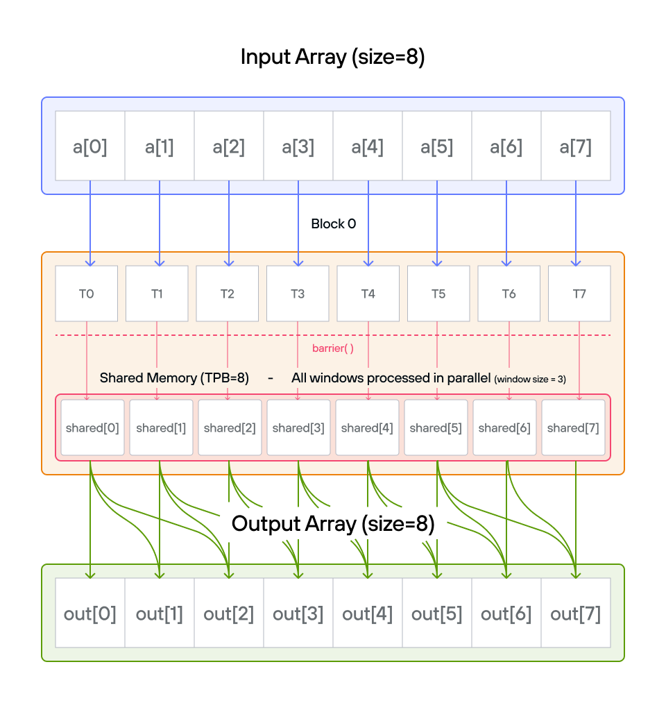
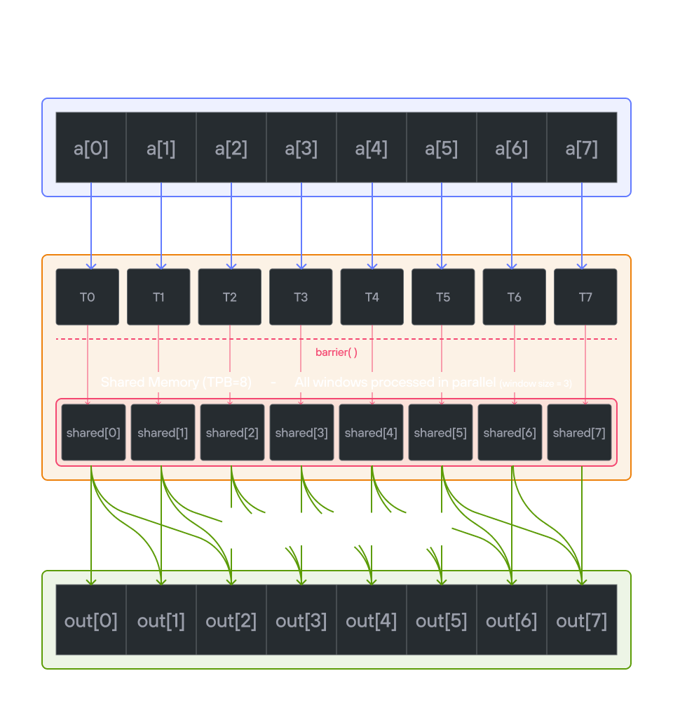
Key concepts

In this puzzle, you’ll learn about:

• Using LayoutTensor for sliding window operations
• Managing shared memory with LayoutTensorBuilder that we saw in puzzle_08
• Efficient neighbor access patterns
• Boundary condition handling

The key insight is how LayoutTensor simplifies shared memory management while maintaining efficient window-based operations.

Configuration

• Array size: SIZE = 8 elements
• Threads per block: TPB = 8
• Window size: 3 elements
• Shared memory: TPB elements

Notes:

• Tensor builder: Use LayoutTensorBuilder[dtype]().row_major[TPB]().shared().alloc()
• Window access: Natural indexing for 3-element windows
• Edge handling: Special cases for first two positions
• Memory pattern: One shared memory load per thread

Code to complete

alias TPB = 8
alias SIZE = 8
alias BLOCKS_PER_GRID = (1, 1)
alias THREADS_PER_BLOCK = (TPB, 1)
alias dtype = DType.float32
alias layout = Layout.row_major(SIZE)


fn pooling[
    layout: Layout
](
    output: LayoutTensor[mut=True, dtype, layout],
    a: LayoutTensor[mut=True, dtype, layout],
    size: Int,
):
    # Allocate shared memory using tensor builder
    shared = tb[dtype]().row_major[TPB]().shared().alloc()

    global_i = block_dim.x * block_idx.x + thread_idx.x
    local_i = thread_idx.x
    # FIX ME IN (roughly 10 lines)

View full file: problems/p11/p11_layout_tensor.mojo

Running the code

To test your solution, run the following command in your terminal:

uv run poe p11_layout_tensor

pixi run p11_layout_tensor

Your output will look like this if the puzzle isn’t solved yet:

out: HostBuffer([0.0, 0.0, 0.0, 0.0, 0.0, 0.0, 0.0, 0.0])
expected: HostBuffer([0.0, 1.0, 3.0, 6.0, 9.0, 12.0, 15.0, 18.0])

Solution

fn pooling[
    layout: Layout
](
    output: LayoutTensor[mut=True, dtype, layout],
    a: LayoutTensor[mut=True, dtype, layout],
    size: Int,
):
    # Allocate shared memory using tensor builder
    shared = tb[dtype]().row_major[TPB]().shared().alloc()

    global_i = block_dim.x * block_idx.x + thread_idx.x
    local_i = thread_idx.x

    # Load data into shared memory
    if global_i < size:
        shared[local_i] = a[global_i]

    # Synchronize threads within block
    barrier()

    # Handle first two special cases
    if global_i == 0:
        output[0] = shared[0]
    elif global_i == 1:
        output[1] = shared[0] + shared[1]
    # Handle general case
    elif 1 < global_i < size:
        output[global_i] = (
            shared[local_i - 2] + shared[local_i - 1] + shared[local_i]
        )

[0.0, 1.0, 3.0, 6.0, 9.0, 12.0, 15.0, 18.0]

Puzzle 12: Dot Product

Overview

Implement a kernel that computes the dot-product of vector a and vector b and stores it in output (single number).

Note: You have 1 thread per position. You only need 2 global reads per thread and 1 global write per thread block.

Implementation approaches

🔰 Raw memory approach

Learn how to implement the reduction with manual memory management and synchronization.

📐 LayoutTensor Version

Use LayoutTensor’s features for efficient reduction and shared memory management.

💡 Note: See how LayoutTensor simplifies efficient memory access patterns.

Overview

Implement a kernel that computes the dot-product of vector a and vector b and stores it in output (single number).

Note: You have 1 thread per position. You only need 2 global reads per thread and 1 global write per thread block.

Key concepts

In this puzzle, you’ll learn about:

• Implementing parallel reduction operations
• Using shared memory for intermediate results
• Coordinating threads for collective operations

The key insight is understanding how to efficiently combine multiple values into a single result using parallel computation and shared memory.

Configuration

• Vector size: SIZE = 8 elements
• Threads per block: TPB = 8
• Number of blocks: 1
• Output size: 1 element
• Shared memory: TPB elements

Notes:

• Element access: Each thread reads corresponding elements from a and b
• Partial results: Computing and storing intermediate values
• Thread coordination: Synchronizing before combining results
• Final reduction: Converting partial results to scalar output

Note: For this problem, you don’t need to worry about number of shared reads. We will handle that challenge later.

Code to complete

alias TPB = 8
alias SIZE = 8
alias BLOCKS_PER_GRID = (1, 1)
alias THREADS_PER_BLOCK = (TPB, 1)
alias dtype = DType.float32


fn dot_product(
    output: UnsafePointer[Scalar[dtype]],
    a: UnsafePointer[Scalar[dtype]],
    b: UnsafePointer[Scalar[dtype]],
    size: Int,
):
    # FILL ME IN (roughly 13 lines)
    ...

View full file: problems/p12/p12.mojo

Running the code

To test your solution, run the following command in your terminal:

uv run poe p12

pixi run p12

Your output will look like this if the puzzle isn’t solved yet:

out: HostBuffer([0.0])
expected: HostBuffer([140.0])

Solution

fn dot_product(
    output: UnsafePointer[Scalar[dtype]],
    a: UnsafePointer[Scalar[dtype]],
    b: UnsafePointer[Scalar[dtype]],
    size: Int,
):
    shared = stack_allocation[
        TPB,
        Scalar[dtype],
        address_space = AddressSpace.SHARED,
    ]()
    global_i = block_dim.x * block_idx.x + thread_idx.x
    local_i = thread_idx.x
    if global_i < size:
        shared[local_i] = a[global_i] * b[global_i]

    barrier()

    # The following causes race condition: all threads writing to the same location
    # out[0] += shared[local_i]

    # Instead can do parallel reduction in shared memory as opposed to
    # global memory which has no guarantee on synchronization.
    # Loops using global memory can cause thread divergence because
    # fundamentally GPUs execute threads in warps (groups of 32 threads typically)
    # and warps can be scheduled independently.
    # However, shared memory does not have such issues as long as we use `barrier()`
    # correctly when we're in the same thread block.
    stride = TPB // 2
    while stride > 0:
        if local_i < stride:
            shared[local_i] += shared[local_i + stride]

        barrier()
        stride //= 2

    # only thread 0 writes the final result
    if local_i == 0:
        output[0] = shared[0]

Thread i: shared[i] = a[i] * b[i]

Initial:  [0*0  1*1  2*2  3*3  4*4  5*5  6*6  7*7]
        = [0    1    4    9    16   25   36   49]

Step 1:   [0+16 1+25 4+36 9+49  16   25   36   49]
        = [16   26   40   58   16   25   36   49]

Step 2:   [16+40 26+58 40   58   16   25   36   49]
        = [56   84   40   58   16   25   36   49]

Step 3:   [56+84  84   40   58   16   25   36   49]
        = [140   84   40   58   16   25   36   49]

Initial shared memory: [0 1 4 9 16 25 36 49]

Step 1 (stride = 4):
Thread 0 reads: shared[0] = 0, shared[4] = 16
Thread 1 reads: shared[1] = 1, shared[5] = 25
Thread 2 reads: shared[2] = 4, shared[6] = 36
Thread 3 reads: shared[3] = 9, shared[7] = 49

Without barrier:
- Thread 0 writes: shared[0] = 0 + 16 = 16
- Thread 1 starts next step (stride = 2) before Thread 0 finishes
  and reads old value shared[0] = 0 instead of 16!

Step 1 (stride = 4):
All threads write their sums:
[16 26 40 58 16 25 36 49]
barrier() ensures ALL threads see these values

Step 2 (stride = 2):
Now threads safely read the updated values:
Thread 0: shared[0] = 16 + 40 = 56
Thread 1: shared[1] = 26 + 58 = 84

Overview

Implement a kernel that computes the dot-product of 1D LayoutTensor a and 1D LayoutTensor b and stores it in 1D LayoutTensor output (single number).

Note: You have 1 thread per position. You only need 2 global reads per thread and 1 global write per thread block.

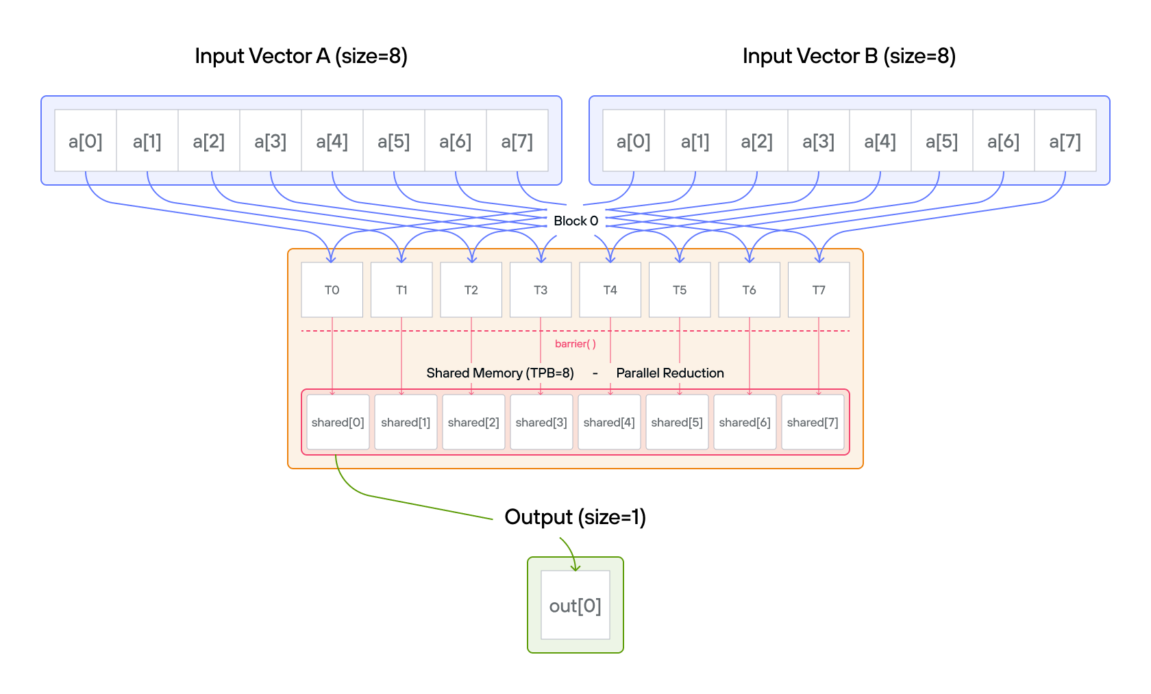
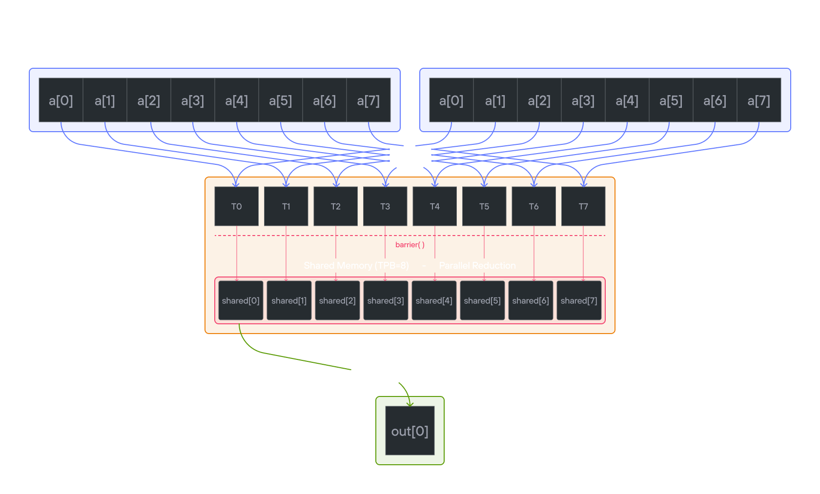
Key concepts

In this puzzle, you’ll learn about:

• Similar to the puzzle 8 and puzzle 11, implementing parallel reduction with LayoutTensor
• Managing shared memory using LayoutTensorBuilder
• Coordinating threads for collective operations
• Using layout-aware tensor operations

The key insight is how LayoutTensor simplifies memory management while maintaining efficient parallel reduction patterns.

Configuration

• Vector size: SIZE = 8 elements
• Threads per block: TPB = 8
• Number of blocks: 1
• Output size: 1 element
• Shared memory: TPB elements

Notes:

• Tensor builder: Use LayoutTensorBuilder[dtype]().row_major[TPB]().shared().alloc()
• Element access: Natural indexing with bounds checking
• Layout handling: Separate layouts for input and output
• Thread coordination: Same synchronization patterns with barrier()

Code to complete

from gpu import thread_idx, block_idx, block_dim, barrier
from layout import Layout, LayoutTensor
from layout.tensor_builder import LayoutTensorBuild as tb


alias TPB = 8
alias SIZE = 8
alias BLOCKS_PER_GRID = (1, 1)
alias THREADS_PER_BLOCK = (TPB, 1)
alias dtype = DType.float32
alias layout = Layout.row_major(SIZE)
alias out_layout = Layout.row_major(1)


fn dot_product[
    in_layout: Layout, out_layout: Layout
](
    output: LayoutTensor[mut=True, dtype, out_layout],
    a: LayoutTensor[mut=True, dtype, in_layout],
    b: LayoutTensor[mut=True, dtype, in_layout],
    size: Int,
):
    # FILL ME IN (roughly 13 lines)
    ...

View full file: problems/p12/p12_layout_tensor.mojo

Running the code

To test your solution, run the following command in your terminal:

uv run poe p12_layout_tensor

pixi run p12_layout_tensor

Your output will look like this if the puzzle isn’t solved yet:

out: HostBuffer([0.0])
expected: HostBuffer([140.0])

Solution

fn dot_product[
    in_layout: Layout, out_layout: Layout
](
    output: LayoutTensor[mut=True, dtype, out_layout],
    a: LayoutTensor[mut=True, dtype, in_layout],
    b: LayoutTensor[mut=True, dtype, in_layout],
    size: Int,
):
    shared = tb[dtype]().row_major[TPB]().shared().alloc()
    global_i = block_dim.x * block_idx.x + thread_idx.x
    local_i = thread_idx.x

    # Compute element-wise multiplication into shared memory
    if global_i < size:
        shared[local_i] = a[global_i] * b[global_i]

    # Synchronize threads within block
    barrier()

    # Parallel reduction in shared memory
    stride = TPB // 2
    while stride > 0:
        if local_i < stride:
            shared[local_i] += shared[local_i + stride]

        barrier()
        stride //= 2

    # Only thread 0 writes the final result
    if local_i == 0:
        output[0] = shared[0]

shared[local_i] = a[global_i] * b[global_i]

Initial:  [0*0  1*1  2*2  3*3  4*4  5*5  6*6  7*7]
        = [0    1    4    9    16   25   36   49]

Step 1:   [0+16 1+25 4+36 9+49  16   25   36   49]
        = [16   26   40   58   16   25   36   49]

Step 2:   [16+40 26+58 40   58   16   25   36   49]
        = [56   84   40   58   16   25   36   49]

Step 3:   [56+84  84   40   58   16   25   36   49]
        = [140   84   40   58   16   25   36   49]

Initial shared memory: [0 1 4 9 16 25 36 49]

Step 1 (stride = 4):
Thread 0 reads: shared[0] = 0, shared[4] = 16
Thread 1 reads: shared[1] = 1, shared[5] = 25
Thread 2 reads: shared[2] = 4, shared[6] = 36
Thread 3 reads: shared[3] = 9, shared[7] = 49

Without barrier:
- Thread 0 writes: shared[0] = 0 + 16 = 16
- Thread 1 starts next step (stride = 2) before Thread 0 finishes
  and reads old value shared[0] = 0 instead of 16!

Step 1 (stride = 4):
All threads write their sums:
[16 26 40 58 16 25 36 49]
barrier() ensures ALL threads see these values

Step 2 (stride = 2):
Now threads safely read the updated values:
Thread 0: shared[0] = 16 + 40 = 56
Thread 1: shared[1] = 26 + 58 = 84

Puzzle 13: 1D Convolution

Moving to LayoutTensor

So far in our GPU puzzle journey, we’ve been exploring two parallel approaches to GPU memory management:

1. Raw memory management with direct pointer manipulation using UnsafePointer
2. The more structured LayoutTensor and its related abstractions such as LayoutTensorBuild

Starting from this puzzle, we’re transitioning exclusively to using LayoutTensor. This abstraction provides several benefits:

• Type-safe memory access patterns
• Clear representation of data layouts
• Better code maintainability
• Reduced chance of memory-related bugs
• More expressive code that better represents the underlying computations
• A lot more … that we’ll uncover gradually!

This transition aligns with best practices in modern GPU programming in Mojo 🔥, where higher-level abstractions help manage complexity without sacrificing performance.

Overview

In signal processing and image analysis, convolution is a fundamental operation that combines two sequences to produce a third sequence. This puzzle challenges you to implement a 1D convolution on the GPU, where each output element is computed by sliding a kernel over an input array.

Implement a kernel that computes a 1D convolution between vector a and vector b and stores it in output using the LayoutTensor abstraction.

Note: You need to handle the general case. You only need 2 global reads and 1 global write per thread.

For those new to convolution, think of it as a weighted sliding window operation. At each position, we multiply the kernel values with the corresponding input values and sum the results. In mathematical notation, this is often written as:

\[\Large output[i] = \sum_{j=0}^{\text{CONV}-1} a[i+j] \cdot b[j] \]

In pseudocode, 1D convolution is:

for i in range(SIZE):
    for j in range(CONV):
        if i + j < SIZE:
            ret[i] += a_host[i + j] * b_host[j]

This puzzle is split into two parts to help you build understanding progressively:

• Simple Version with Single Block Start here to learn the basics of implementing convolution with shared memory in a single block using LayoutTensor.

• Block Boundary Version Then tackle the more challenging case where data needs to be shared across block boundaries, leveraging LayoutTensor’s capabilities.

Each version presents unique challenges in terms of memory access patterns and thread coordination. The simple version helps you understand the basic convolution operation, while the complete version tests your ability to handle more complex scenarios that arise in real-world GPU programming.

Simple Case with Single Block

Implement a kernel that computes a 1D convolution between 1D LayoutTensor a and 1D LayoutTensor b and stores it in 1D LayoutTensor `output.

Note: You need to handle the general case. You only need 2 global reads and 1 global write per thread.

Key concepts

In this puzzle, you’ll learn about:

• Implementing sliding window operations on GPUs
• Managing data dependencies across threads
• Using shared memory for overlapping regions

The key insight is understanding how to efficiently access overlapping elements while maintaining correct boundary conditions.

Configuration

• Input array size: SIZE = 6 elements
• Kernel size: CONV = 3 elements
• Threads per block: TPB = 8
• Number of blocks: 1
• Shared memory: Two arrays of size SIZE and CONV

Notes:

• Data loading: Each thread loads one element from input and kernel
• Memory pattern: Shared arrays for input and convolution kernel
• Thread sync: Coordination before computation

Code to complete

alias TPB = 8
alias SIZE = 6
alias CONV = 3
alias BLOCKS_PER_GRID = (1, 1)
alias THREADS_PER_BLOCK = (TPB, 1)
alias dtype = DType.float32
alias in_layout = Layout.row_major(SIZE)
alias out_layout = Layout.row_major(SIZE)
alias conv_layout = Layout.row_major(CONV)


fn conv_1d_simple[
    in_layout: Layout, out_layout: Layout, conv_layout: Layout
](
    output: LayoutTensor[mut=False, dtype, out_layout],
    a: LayoutTensor[mut=False, dtype, in_layout],
    b: LayoutTensor[mut=False, dtype, conv_layout],
):
    global_i = block_dim.x * block_idx.x + thread_idx.x
    local_i = thread_idx.x
    # FILL ME IN (roughly 14 lines)

View full file: problems/p13/p13.mojo

Running the code

To test your solution, run the following command in your terminal:

uv run poe p13 --simple

pixi run p13 --simple

Your output will look like this if the puzzle isn’t solved yet:

out: HostBuffer([0.0, 0.0, 0.0, 0.0, 0.0, 0.0])
expected: HostBuffer([5.0, 8.0, 11.0, 14.0, 5.0, 0.0])

Solution

fn conv_1d_simple[
    in_layout: Layout, out_layout: Layout, conv_layout: Layout
](
    output: LayoutTensor[mut=False, dtype, out_layout],
    a: LayoutTensor[mut=False, dtype, in_layout],
    b: LayoutTensor[mut=False, dtype, conv_layout],
):
    global_i = block_dim.x * block_idx.x + thread_idx.x
    local_i = thread_idx.x
    shared_a = tb[dtype]().row_major[SIZE]().shared().alloc()
    shared_b = tb[dtype]().row_major[CONV]().shared().alloc()
    if global_i < SIZE:
        shared_a[local_i] = a[global_i]

    if global_i < CONV:
        shared_b[local_i] = b[global_i]

    barrier()

    # Note: this is unsafe as it enforces no guard so could access `shared_a` beyond its bounds
    # local_sum = Scalar[dtype](0)
    # for j in range(CONV):
    #     if local_i + j < SIZE:
    #         local_sum += shared_a[local_i + j] * shared_b[j]

    # if global_i < SIZE:
    #     out[global_i] = local_sum

    # Safe and correct:
    if global_i < SIZE:
        # Note: using `var` allows us to include the type in the type inference
        # `out.element_type` is available in LayoutTensor
        var local_sum: output.element_type = 0

        # Note: `@parameter` decorator unrolls the loop at compile time given `CONV` is a compile-time constant
        # See: https://docs.modular.com/mojo/manual/decorators/parameter/#parametric-for-statement
        @parameter
        for j in range(CONV):
            # Bonus: do we need this check for this specific example with fixed SIZE, CONV
            if local_i + j < SIZE:
                local_sum += shared_a[local_i + j] * shared_b[j]

        output[global_i] = local_sum

Input array a:   [0  1  2  3  4  5]
Kernel b:        [0  1  2]

Block Boundary Version

Implement a kernel that computes a 1D convolution between 1D LayoutTensor a and 1D LayoutTensor b and stores it in 1D LayoutTensor output.

Note: You need to handle the general case. You only need 2 global reads and 1 global write per thread.

Configuration

• Input array size: SIZE_2 = 15 elements
• Kernel size: CONV_2 = 4 elements
• Threads per block: TPB = 8
• Number of blocks: 2
• Shared memory: TPB + CONV_2 - 1 elements for input

Notes:

• Extended loading: Account for boundary overlap
• Block edges: Handle data across block boundaries
• Memory layout: Efficient shared memory usage
• Synchronization: Proper thread coordination

Code to complete

alias SIZE_2 = 15
alias CONV_2 = 4
alias BLOCKS_PER_GRID_2 = (2, 1)
alias THREADS_PER_BLOCK_2 = (TPB, 1)
alias in_2_layout = Layout.row_major(SIZE_2)
alias out_2_layout = Layout.row_major(SIZE_2)
alias conv_2_layout = Layout.row_major(CONV_2)


fn conv_1d_block_boundary[
    in_layout: Layout, out_layout: Layout, conv_layout: Layout, dtype: DType
](
    output: LayoutTensor[mut=False, dtype, out_layout],
    a: LayoutTensor[mut=False, dtype, in_layout],
    b: LayoutTensor[mut=False, dtype, conv_layout],
):
    global_i = block_dim.x * block_idx.x + thread_idx.x
    local_i = thread_idx.x
    # FILL ME IN (roughly 18 lines)

View full file: problems/p13/p13.mojo

Running the code

To test your solution, run the following command in your terminal:

uv run poe p13 --block-boundary

pixi run p13 --block-boundary

Your output will look like this if the puzzle isn’t solved yet:

out: HostBuffer([0.0, 0.0, 0.0, 0.0, 0.0, 0.0, 0.0, 0.0, 0.0, 0.0, 0.0, 0.0, 0.0, 0.0, 0.0])
expected: HostBuffer([14.0, 20.0, 26.0, 32.0, 38.0, 44.0, 50.0, 56.0, 62.0, 68.0, 74.0, 80.0, 41.0, 14.0, 0.0])

Solution

fn conv_1d_block_boundary[
    in_layout: Layout, out_layout: Layout, conv_layout: Layout, dtype: DType
](
    output: LayoutTensor[mut=False, dtype, out_layout],
    a: LayoutTensor[mut=False, dtype, in_layout],
    b: LayoutTensor[mut=False, dtype, conv_layout],
):
    global_i = block_dim.x * block_idx.x + thread_idx.x
    local_i = thread_idx.x
    # first: need to account for padding
    shared_a = tb[dtype]().row_major[TPB + CONV_2 - 1]().shared().alloc()
    shared_b = tb[dtype]().row_major[CONV_2]().shared().alloc()
    if global_i < SIZE_2:
        shared_a[local_i] = a[global_i]
    else:
        shared_a[local_i] = 0

    # second: load elements needed for convolution at block boundary
    if local_i < CONV_2 - 1:
        # indices from next block
        next_idx = global_i + TPB
        if next_idx < SIZE_2:
            shared_a[TPB + local_i] = a[next_idx]
        else:
            # Initialize out-of-bounds elements to 0 to avoid reading from uninitialized memory
            # which is an undefined behavior
            shared_a[TPB + local_i] = 0

    if local_i < CONV_2:
        shared_b[local_i] = b[local_i]

    barrier()

    if global_i < SIZE_2:
        var local_sum: output.element_type = 0

        @parameter
        for j in range(CONV_2):
            if global_i + j < SIZE_2:
                local_sum += shared_a[local_i + j] * shared_b[j]

        output[global_i] = local_sum

Test Configuration:
- Full array size: SIZE_2 = 15 elements
- Grid: 2 blocks × 8 threads
- Convolution kernel: CONV_2 = 4 elements

Block 0 shared memory:  [0 1 2 3 4 5 6 7|8 9 10]  // TPB(8) + (CONV_2-1)(3) padding
Block 1 shared memory:  [8 9 10 11 12 13 14|0 0]  // Second block with padding

Size calculation:
- Main data: TPB elements (8)
- Overlap: CONV_2 - 1 elements (4 - 1 = 3)
- Total: TPB + CONV_2 - 1 = 8 + 4 - 1 = 11 elements

Puzzle 14: Prefix Sum

Overview

Prefix sum (also known as scan) is a fundamental parallel algorithm that computes running totals of a sequence. Found at the heart of many parallel applications - from sorting algorithms to scientific simulations - it transforms a sequence of numbers into their running totals. While simple to compute sequentially, making this efficient on a GPU requires clever parallel thinking!

Implement a kernel that computes a prefix-sum over 1D LayoutTensor a and stores it in 1D LayoutTensor output.

Note: If the size of a is greater than the block size, only store the sum of each block.

Key concepts

In this puzzle, you’ll learn about:

• Parallel algorithms with logarithmic complexity
• Shared memory coordination patterns
• Multi-phase computation strategies

The key insight is understanding how to transform a sequential operation into an efficient parallel algorithm using shared memory.

For example, given an input sequence \([3, 1, 4, 1, 5, 9]\), the prefix sum would produce:

• \([3]\) (just the first element)
• \([3, 4]\) (3 + 1)
• \([3, 4, 8]\) (previous sum + 4)
• \([3, 4, 8, 9]\) (previous sum + 1)
• \([3, 4, 8, 9, 14]\) (previous sum + 5)
• \([3, 4, 8, 9, 14, 23]\) (previous sum + 9)

Mathematically, for a sequence \([x_0, x_1, …, x_n]\), the prefix sum produces: \[ [x_0, x_0+x_1, x_0+x_1+x_2, …, \sum_{i=0}^n x_i] \]

While a sequential algorithm would need \(O(n)\) steps, our parallel approach will use a clever two-phase algorithm that completes in \(O(\log n)\) steps! Here’s a visualization of this process:

This puzzle is split into two parts to help you master the concept:

• Simple Version Start with a single block implementation where all data fits in shared memory. This helps understand the core parallel algorithm.

• Complete Version Then tackle the more challenging case of handling larger arrays that span multiple blocks, requiring coordination between blocks.

Each version builds on the previous one, helping you develop a deep understanding of parallel prefix sum computation. The simple version establishes the fundamental algorithm, while the complete version shows how to scale it to larger datasets - a common requirement in real-world GPU applications.

Simple Version

Implement a kernel that computes a prefix-sum over 1D LayoutTensor a and stores it in 1D LayoutTensor output.

Note: If the size of a is greater than the block size, only store the sum of each block.

Configuration

• Array size: SIZE = 8 elements
• Threads per block: TPB = 8
• Number of blocks: 1
• Shared memory: TPB elements

Notes:

• Data loading: Each thread loads one element using LayoutTensor access
• Memory pattern: Shared memory for intermediate results using LayoutTensorBuild
• Thread sync: Coordination between computation phases
• Access pattern: Stride-based parallel computation
• Type safety: Leveraging LayoutTensor’s type system

Code to complete

alias TPB = 8
alias SIZE = 8
alias BLOCKS_PER_GRID = (1, 1)
alias THREADS_PER_BLOCK = (TPB, 1)
alias dtype = DType.float32
alias layout = Layout.row_major(SIZE)


fn prefix_sum_simple[
    layout: Layout
](
    output: LayoutTensor[mut=False, dtype, layout],
    a: LayoutTensor[mut=False, dtype, layout],
    size: Int,
):
    global_i = block_dim.x * block_idx.x + thread_idx.x
    local_i = thread_idx.x
    # FILL ME IN (roughly 18 lines)

View full file: problems/p14/p14.mojo

Running the code

To test your solution, run the following command in your terminal:

uv run poe p14 --simple

pixi run p14 --simple

Your output will look like this if the puzzle isn’t solved yet:

out: DeviceBuffer([0.0, 0.0, 0.0, 0.0, 0.0, 0.0, 0.0, 0.0])
expected: HostBuffer([0.0, 1.0, 3.0, 6.0, 10.0, 15.0, 21.0, 28.0])

Solution

fn prefix_sum_simple[
    layout: Layout
](
    output: LayoutTensor[mut=False, dtype, layout],
    a: LayoutTensor[mut=False, dtype, layout],
    size: Int,
):
    global_i = block_dim.x * block_idx.x + thread_idx.x
    local_i = thread_idx.x
    shared = tb[dtype]().row_major[TPB]().shared().alloc()
    if global_i < size:
        shared[local_i] = a[global_i]

    barrier()

    offset = 1
    for i in range(Int(log2(Scalar[dtype](TPB)))):
        var current_val: output.element_type = 0
        if local_i >= offset and local_i < size:
            current_val = shared[local_i - offset]  # read

        barrier()
        if local_i >= offset and local_i < size:
            shared[local_i] += current_val

        barrier()
        offset *= 2

    if global_i < size:
        output[global_i] = shared[local_i]

Threads:      T₀   T₁   T₂   T₃   T₄   T₅   T₆   T₇
Input array:  [0    1    2    3    4    5    6    7]
shared:       [0    1    2    3    4    5    6    7]
               ↑    ↑    ↑    ↑    ↑    ↑    ↑    ↑
              T₀   T₁   T₂   T₃   T₄   T₅   T₆   T₇

T₁ reads shared[0] = 0    T₅ reads shared[4] = 4
T₂ reads shared[1] = 1    T₆ reads shared[5] = 5
T₃ reads shared[2] = 2    T₇ reads shared[6] = 6
T₄ reads shared[3] = 3

Before:      [0    1    2    3    4    5    6    7]
Add:              +0   +1   +2   +3   +4   +5   +6
                   |    |    |    |    |    |    |
Result:      [0    1    3    5    7    9    11   13]
                   ↑    ↑    ↑    ↑    ↑    ↑    ↑
                  T₁   T₂   T₃   T₄   T₅   T₆   T₇

T₂ reads shared[0] = 0    T₅ reads shared[3] = 5
T₃ reads shared[1] = 1    T₆ reads shared[4] = 7
T₄ reads shared[2] = 3    T₇ reads shared[5] = 9

Before:      [0    1    3    5    7    9    11   13]
Add:                   +0   +1   +3   +5   +7   +9
                        |    |    |    |    |    |
Result:      [0    1    3    6    10   14   18   22]
                        ↑    ↑    ↑    ↑    ↑    ↑
                       T₂   T₃   T₄   T₅   T₆   T₇

T₄ reads shared[0] = 0    T₆ reads shared[2] = 3
T₅ reads shared[1] = 1    T₇ reads shared[3] = 6

Before:      [0    1    3    6    10   14   18   22]
Add:                              +0   +1   +3   +6
                                  |    |    |    |
Result:      [0    1    3    6    10   15   21   28]
                                  ↑    ↑    ↑    ↑
                                  T₄   T₅   T₆   T₇

Threads:      T₀   T₁   T₂   T₃   T₄   T₅   T₆   T₇
global_i:     0    1    2    3    4    5    6    7
output:       [0    1    3    6    10   15   21   28]
              ↑    ↑    ↑    ↑    ↑    ↑    ↑    ↑
              T₀   T₁   T₂   T₃   T₄   T₅   T₆   T₇

Complete Version

Implement a kernel that computes a prefix-sum over 1D LayoutTensor a and stores it in 1D LayoutTensor output.

Note: If the size of a is greater than the block size, we need to synchronize across multiple blocks to get the correct result.

Configuration

• Array size: SIZE_2 = 15 elements
• Threads per block: TPB = 8
• Number of blocks: 2
• Shared memory: TPB elements per block

Notes:

• Multiple blocks: When the input array is larger than one block, we need a multi-phase approach
• Block-level sync: Within a block, use barrier() to synchronize threads
• Host-level sync: Between blocks, use ctx.synchronize() at the host level
• Auxiliary storage: Use extra space to store block sums for cross-block communication

Code to complete

You need to complete two separate kernel functions for the multi-block prefix sum:

1. First kernel (prefix_sum_local_phase): Computes local prefix sums within each block and stores block sums
2. Second kernel (prefix_sum_block_sum_phase): Adds previous block sums to elements in subsequent blocks

The main function will handle the necessary host-side synchronization between these kernels.

alias SIZE_2 = 15
alias BLOCKS_PER_GRID_2 = (2, 1)
alias THREADS_PER_BLOCK_2 = (TPB, 1)
alias EXTENDED_SIZE = SIZE_2 + 2  # up to 2 blocks
alias extended_layout = Layout.row_major(EXTENDED_SIZE)


# Kernel 1: Compute local prefix sums and store block sums in out
fn prefix_sum_local_phase[
    out_layout: Layout, in_layout: Layout
](
    output: LayoutTensor[mut=False, dtype, out_layout],
    a: LayoutTensor[mut=False, dtype, in_layout],
    size: Int,
):
    global_i = block_dim.x * block_idx.x + thread_idx.x
    local_i = thread_idx.x
    # FILL ME IN (roughly 20 lines)


# Kernel 2: Add block sums to their respective blocks
fn prefix_sum_block_sum_phase[
    layout: Layout
](output: LayoutTensor[mut=False, dtype, layout], size: Int):
    global_i = block_dim.x * block_idx.x + thread_idx.x
    # FILL ME IN (roughly 3 lines)

View full file: problems/p14/p14.mojo

The key to this puzzle is understanding that barrier only synchronizes threads within a block, not across blocks. For cross-block synchronization, you need to use host-level synchronization:

            # Phase 1: Local prefix sums
            ctx.enqueue_function[
                prefix_sum_local_phase[extended_layout, extended_layout]
            ](
                out_tensor,
                a_tensor,
                size,
                grid_dim=BLOCKS_PER_GRID_2,
                block_dim=THREADS_PER_BLOCK_2,
            )

            # Phase 2: Add block sums
            ctx.enqueue_function[prefix_sum_block_sum_phase[extended_layout]](
                out_tensor,
                size,
                grid_dim=BLOCKS_PER_GRID_2,
                block_dim=THREADS_PER_BLOCK_2,
            )

Simple version (single block): [0,1,2,3,4,5,6,7] → [0,1,3,6,10,15,21,28]

Complete version (two blocks):
Block 0: [0,1,2,3,4,5,6,7] → [0,1,3,6,10,15,21,28]
Block 1: [8,9,10,11,12,13,14] → [8,17,27,38,50,63,77]

After first phase: [0,1,3,6,10,15,21,28, 8,17,27,38,50,63,77, ???,???]

Running the code

To test your solution, run the following command in your terminal:

uv run poe p14 --complete

pixi run p14 --complete

Your output will look like this if the puzzle isn’t solved yet:

out: HostBuffer([0.0, 0.0, 0.0, 0.0, 0.0, 0.0, 0.0, 0.0, 0.0, 0.0, 0.0, 0.0, 0.0, 0.0, 0.0, 0.0, 0.0])
expected: HostBuffer([0.0, 1.0, 3.0, 6.0, 10.0, 15.0, 21.0, 28.0, 36.0, 45.0, 55.0, 66.0, 78.0, 91.0, 105.0])

Solution

# Kernel 1: Compute local prefix sums and store block sums in out
fn prefix_sum_local_phase[
    out_layout: Layout, in_layout: Layout
](
    output: LayoutTensor[mut=False, dtype, out_layout],
    a: LayoutTensor[mut=False, dtype, in_layout],
    size: Int,
):
    global_i = block_dim.x * block_idx.x + thread_idx.x
    local_i = thread_idx.x
    shared = tb[dtype]().row_major[TPB]().shared().alloc()

    # Load data into shared memory
    # Example with SIZE_2=15, TPB=8, BLOCKS=2:
    # Block 0 shared mem: [0,1,2,3,4,5,6,7]
    # Block 1 shared mem: [8,9,10,11,12,13,14,uninitialized]
    # Note: The last position remains uninitialized since global_i >= size,
    # but this is safe because that thread doesn't participate in computation
    if global_i < size:
        shared[local_i] = a[global_i]

    barrier()

    # Compute local prefix sum using parallel reduction
    # This uses a tree-based algorithm with log(TPB) iterations
    # Iteration 1 (offset=1):
    #   Block 0: [0,0+1,2+1,3+2,4+3,5+4,6+5,7+6] = [0,1,3,5,7,9,11,13]
    # Iteration 2 (offset=2):
    #   Block 0: [0,1,3+0,5+1,7+3,9+5,11+7,13+9] = [0,1,3,6,10,14,18,22]
    # Iteration 3 (offset=4):
    #   Block 0: [0,1,3,6,10+0,14+1,18+3,22+6] = [0,1,3,6,10,15,21,28]
    #   Block 1 follows same pattern to get [8,17,27,38,50,63,77,???]
    offset = 1
    for i in range(Int(log2(Scalar[dtype](TPB)))):
        var current_val: output.element_type = 0
        if local_i >= offset and local_i < TPB:
            current_val = shared[local_i - offset]  # read

        barrier()
        if local_i >= offset and local_i < TPB:
            shared[local_i] += current_val  # write

        barrier()
        offset *= 2

    # Write local results to output
    # Block 0 writes: [0,1,3,6,10,15,21,28]
    # Block 1 writes: [8,17,27,38,50,63,77,???]
    if global_i < size:
        output[global_i] = shared[local_i]

    # Store block sums in auxiliary space
    # Block 0: Thread 7 stores shared[7] == 28 at position size+0 (position 15)
    # Block 1: Thread 7 stores shared[7] == ??? at position size+1 (position 16).  This sum is not needed for the final output.
    # This gives us: [0,1,3,6,10,15,21,28, 8,17,27,38,50,63,77, 28,???]
    #                                                           ↑  ↑
    #                                                     Block sums here
    if local_i == TPB - 1:
        output[size + block_idx.x] = shared[local_i]


# Kernel 2: Add block sums to their respective blocks
fn prefix_sum_block_sum_phase[
    layout: Layout
](output: LayoutTensor[mut=False, dtype, layout], size: Int):
    global_i = block_dim.x * block_idx.x + thread_idx.x

    # Second pass: add previous block's sum to each element
    # Block 0: No change needed - already correct
    # Block 1: Add Block 0's sum (28) to each element
    #   Before: [8,17,27,38,50,63,77]
    #   After: [36,45,55,66,78,91,105]
    # Final result combines both blocks:
    # [0,1,3,6,10,15,21,28, 36,45,55,66,78,91,105]
    if block_idx.x > 0 and global_i < size:
        prev_block_sum = output[size + block_idx.x - 1]
        output[global_i] += prev_block_sum

Input array:  [0, 1, 2, 3, 4, 5, 6, 7, 8, 9, 10, 11, 12, 13, 14]

Block 0 processes: [0, 1, 2, 3, 4, 5, 6, 7]
Block 1 processes: [8, 9, 10, 11, 12, 13, 14] (7 valid elements)

Extended buffer: [data values (15 elements)] + [block sums (2 elements)]
                 [0...14] + [block0_sum, block1_sum]

[0, 1, 3, 6, 10, 15, 21, 28, 8, 17, 27, 38, 50, 63, 77, 28, ???]
                                                        ^   ^
                                                Block sums stored here

# Phase 1: Local prefix sums
ctx.enqueue_function[prefix_sum_local_phase[...]](...)

# Phase 2: Add block sums (automatically waits for Phase 1)
ctx.enqueue_function[prefix_sum_block_sum_phase[...]](...)

# After both kernels complete, before reading results on host
ctx.synchronize()  # Host waits for GPU to finish

with out.map_to_host() as out_host:  # Now safe to read GPU results
    print("out:", out_host)

Puzzle 15: Axis Sum

Overview

Implement a kernel that computes a sum over each row of 2D matrix a and stores it in output using LayoutTensor.

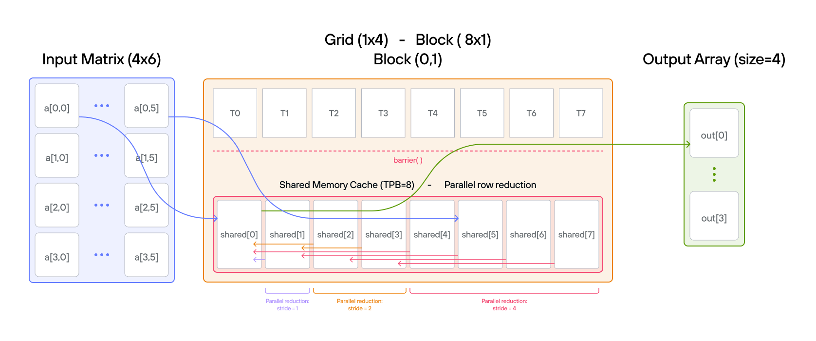
Key concepts

In this puzzle, you’ll learn about:

• Parallel reduction along matrix dimensions using LayoutTensor
• Using block coordinates for data partitioning
• Efficient shared memory reduction patterns
• Working with multi-dimensional tensor layouts

The key insight is understanding how to map thread blocks to matrix rows and perform efficient parallel reduction within each block while leveraging LayoutTensor’s dimensional indexing.

Configuration

• Matrix dimensions: \(\text{BATCH} \times \text{SIZE} = 4 \times 6\)
• Threads per block: \(\text{TPB} = 8\)
• Grid dimensions: \(1 \times \text{BATCH}\)
• Shared memory: \(\text{TPB}\) elements per block
• Input layout: Layout.row_major(BATCH, SIZE)
• Output layout: Layout.row_major(BATCH, 1)

Matrix visualization:

Row 0: [0, 1, 2, 3, 4, 5]       → Block(0,0)
Row 1: [6, 7, 8, 9, 10, 11]     → Block(0,1)
Row 2: [12, 13, 14, 15, 16, 17] → Block(0,2)
Row 3: [18, 19, 20, 21, 22, 23] → Block(0,3)

Code to Complete

from gpu import thread_idx, block_idx, block_dim, barrier
from layout import Layout, LayoutTensor
from layout.tensor_builder import LayoutTensorBuild as tb


alias TPB = 8
alias BATCH = 4
alias SIZE = 6
alias BLOCKS_PER_GRID = (1, BATCH)
alias THREADS_PER_BLOCK = (TPB, 1)
alias dtype = DType.float32
alias in_layout = Layout.row_major(BATCH, SIZE)
alias out_layout = Layout.row_major(BATCH, 1)


fn axis_sum[
    in_layout: Layout, out_layout: Layout
](
    output: LayoutTensor[mut=False, dtype, out_layout],
    a: LayoutTensor[mut=False, dtype, in_layout],
    size: Int,
):
    global_i = block_dim.x * block_idx.x + thread_idx.x
    local_i = thread_idx.x
    batch = block_idx.y
    # FILL ME IN (roughly 15 lines)

View full file: problems/p15/p15.mojo

Running the Code

To test your solution, run the following command in your terminal:

uv run poe p15

pixi run p15

Your output will look like this if the puzzle isn’t solved yet:

out: DeviceBuffer([0.0, 0.0, 0.0, 0.0])
expected: HostBuffer([15.0, 51.0, 87.0, 123.0])

Solution

fn axis_sum[
    in_layout: Layout, out_layout: Layout
](
    output: LayoutTensor[mut=False, dtype, out_layout],
    a: LayoutTensor[mut=False, dtype, in_layout],
    size: Int,
):
    global_i = block_dim.x * block_idx.x + thread_idx.x
    local_i = thread_idx.x
    batch = block_idx.y
    cache = tb[dtype]().row_major[TPB]().shared().alloc()

    # Visualize:
    # Block(0,0): [T0,T1,T2,T3,T4,T5,T6,T7] -> Row 0: [0,1,2,3,4,5]
    # Block(0,1): [T0,T1,T2,T3,T4,T5,T6,T7] -> Row 1: [6,7,8,9,10,11]
    # Block(0,2): [T0,T1,T2,T3,T4,T5,T6,T7] -> Row 2: [12,13,14,15,16,17]
    # Block(0,3): [T0,T1,T2,T3,T4,T5,T6,T7] -> Row 3: [18,19,20,21,22,23]

    # each row is handled by each block bc we have grid_dim=(1, BATCH)

    if local_i < size:
        cache[local_i] = a[batch, local_i]
    else:
        # Add zero-initialize padding elements for later reduction
        cache[local_i] = 0

    barrier()

    # do reduction sum per each block
    stride = TPB // 2
    while stride > 0:
        # Read phase: all threads read the values they need first to avoid race conditions
        var temp_val: output.element_type = 0
        if local_i < stride:
            temp_val = cache[local_i + stride]

        barrier()

        # Write phase: all threads safely write their computed values
        if local_i < stride:
            cache[local_i] += temp_val

        barrier()
        stride //= 2

    # writing with local thread = 0 that has the sum for each batch
    if local_i == 0:
        output[batch, 0] = cache[0]

Input Matrix (4×6) with LayoutTensor:                Block Assignment:
[[ a[0,0]  a[0,1]  a[0,2]  a[0,3]  a[0,4]  a[0,5] ] → Block(0,0)
 [ a[1,0]  a[1,1]  a[1,2]  a[1,3]  a[1,4]  a[1,5] ] → Block(0,1)
 [ a[2,0]  a[2,1]  a[2,2]  a[2,3]  a[2,4]  a[2,5] ] → Block(0,2)
 [ a[3,0]  a[3,1]  a[3,2]  a[3,3]  a[3,4]  a[3,5] ] → Block(0,3)

Puzzle 16: Matrix Multiplication (MatMul)

Overview

Matrix multiplication is a fundamental operation in scientific computing, machine learning, and graphics. Given two matrices \(A\) and \(B\), we want to compute their product \(C = A \times B.\)

For matrices \(A_{m\times k}\) and \(B_{k\times n}\), each element of the result \(C_{m\times n}\) is computed as:

\[\Large C_{ij} = \sum_{l=0}^{k-1} A_{il} \cdot B_{lj} \]

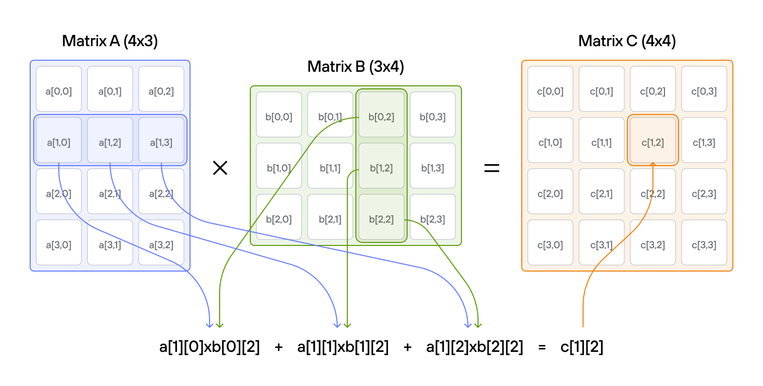
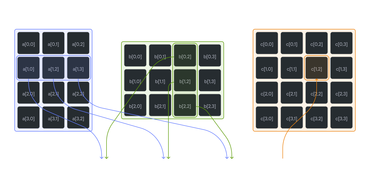
This puzzle explores different approaches to implementing matrix multiplication on GPUs, each with its own performance characteristics:

• Naive Version The straightforward implementation where each thread computes one element of the output matrix. While simple to understand, this approach makes many redundant memory accesses.

• Shared Memory Version Improves performance by loading blocks of input matrices into fast shared memory, reducing global memory accesses. Each thread still computes one output element but reads from shared memory.

• Tiled Version Further optimizes by dividing the computation into tiles, allowing threads to cooperate on loading and computing blocks of the output matrix. This approach better utilizes memory hierarchy and thread cooperation.

Each version builds upon the previous one, introducing new optimization techniques common in GPU programming. You’ll learn how different memory access patterns and thread cooperation strategies affect performance.

The progression illustrates a common pattern in GPU optimization:

1. Start with a correct but naive implementation
2. Reduce global memory access with shared memory
3. Improve data locality and thread cooperation with tiling
4. Use high-level abstractions while maintaining performance

Choose a version to begin your matrix multiplication journey!

Naïve Matrix Multiplication

Overview

Implement a kernel that multiplies square matrices \(A\) and \(B\) and stores the result in \(\text{output}\). This is the most straightforward implementation where each thread computes one element of the output matrix.

Key concepts

In this puzzle, you’ll learn about:

• 2D thread organization for matrix operations
• Global memory access patterns
• Matrix indexing in row-major layout
• Thread-to-output element mapping

The key insight is understanding how to map 2D thread indices to matrix elements and compute dot products in parallel.

Configuration

• Matrix size: \(\text{SIZE} \times \text{SIZE} = 2 \times 2\)
• Threads per block: \(\text{TPB} \times \text{TPB} = 3 \times 3\)
• Grid dimensions: \(1 \times 1\)

Layout configuration:

• Input A: Layout.row_major(SIZE, SIZE)
• Input B: Layout.row_major(SIZE, SIZE)
• Output: Layout.row_major(SIZE, SIZE)

Code to complete

from gpu import thread_idx, block_idx, block_dim, barrier
from layout import Layout, LayoutTensor
from layout.tensor_builder import LayoutTensorBuild as tb


alias TPB = 3
alias SIZE = 2
alias BLOCKS_PER_GRID = (1, 1)
alias THREADS_PER_BLOCK = (TPB, TPB)
alias dtype = DType.float32
alias layout = Layout.row_major(SIZE, SIZE)


fn naive_matmul[
    layout: Layout, size: Int
](
    output: LayoutTensor[mut=False, dtype, layout],
    a: LayoutTensor[mut=False, dtype, layout],
    b: LayoutTensor[mut=False, dtype, layout],
):
    row = block_dim.y * block_idx.y + thread_idx.y
    col = block_dim.x * block_idx.x + thread_idx.x
    # FILL ME IN (roughly 6 lines)

View full file: problems/p16/p16.mojo

Running the code

To test your solution, run the following command in your terminal:

uv run poe p16 --naive

pixi run p16 --naive

Your output will look like this if the puzzle isn’t solved yet:

out: HostBuffer([0.0, 0.0, 0.0, 0.0])
expected: HostBuffer([4.0, 6.0, 12.0, 22.0])

Solution

fn naive_matmul[
    layout: Layout, size: Int
](
    output: LayoutTensor[mut=False, dtype, layout],
    a: LayoutTensor[mut=False, dtype, layout],
    b: LayoutTensor[mut=False, dtype, layout],
):
    row = block_dim.y * block_idx.y + thread_idx.y
    col = block_dim.x * block_idx.x + thread_idx.x

    if row < size and col < size:
        var acc: output.element_type = 0

        @parameter
        for k in range(size):
            acc += a[row, k] * b[k, col]

        output[row, col] = acc

Matrix A:          Matrix B:                   Output C:
[a[0,0] a[0,1]]    [b[0,0] b[0,1]]             [c[0,0] c[0,1]]
[a[1,0] a[1,1]]    [b[1,0] b[1,1]]             [c[1,0] c[1,1]]

Understanding GPU Performance: The Roofline Model

Having implemented the naive matrix multiplication, you might be wondering: How well is our kernel actually performing? Is it limited by the GPU’s computational power, or is something else holding it back?

The roofline model is your compass for GPU optimization—it reveals which hardware bottleneck limits your kernel’s performance and guides you toward the most impactful optimizations. Rather than guessing at improvements, the roofline model shows you exactly where to focus your efforts.

1. Two ceilings for every GPU kernel

Every GPU kernel operates under two fundamental constraints:

• Compute ceiling – how quickly the cores can execute floating-point operations (peak FLOPs/s)
• Memory ceiling – how quickly the memory system can feed those cores with data (peak bytes/s)

Understanding which ceiling constrains your kernel is crucial for optimization strategy. The roofline model visualizes this relationship by plotting two key metrics:

X-axis: Arithmetic Intensity – How much computation you extract per byte of data

\[\Large I = \frac{\text{Total FLOPs}}{\text{Total Bytes from Memory}} \quad [\text{FLOP/B}]\]

Y-axis: Sustained Performance – How fast your kernel actually runs

\[\Large P_{\text{sustained}} = \frac{\text{Total FLOPs}}{\text{Elapsed Time}} \quad [\text{GFLOP/s}]\]

Two “roofs” bound all achievable performance:

The critical intensity

\[\Large I^* = \frac{P_{\text{peak}}}{B_{\text{peak}}}\]

marks where a kernel transitions from memory-bound (\(I < I^* \)) to compute-bound (\(I > I^* \)).

2. Hardware example: NVIDIA A100 specifications

Let’s ground this theory in concrete numbers using the NVIDIA A100:

Peak FP32 throughput \[\Large P_{\text{peak}} = 19.5 \text{ TFLOP/s} = 19{,}500 \text{ GFLOP/s}\]

Peak HBM2 bandwidth \[\Large B_{\text{peak}} = 1{,}555 \text{ GB/s}\]

Critical intensity \[\Large I^* = \frac{19{,}500}{1{,}555} \approx 12.5 \text{ FLOP/B}\]

Source: NVIDIA A100 Tensor Core GPU Architecture

This means kernels with arithmetic intensity below 12.5 FLOP/B are memory-bound, while those above are compute-bound.

3. Visualizing our matrix multiplication implementations

The animation below shows how our puzzle implementations map onto the A100’s roofline model:

The visualization demonstrates the optimization journey we’ll take in this puzzle:

1. Hardware constraints – The red memory roof and blue compute roof define performance limits
2. Our starting point – The naive implementation (left purple dot) sitting firmly on the memory roof
3. Optimization target – The shared memory version (right purple dot) with improved arithmetic intensity
4. Ultimate goal – The golden arrow pointing toward the critical intensity where kernels become compute-bound

4. Analyzing our naive implementation

Let’s examine why our naive kernel from the previous section performs as it does. For our \(2 \times 2\) matrix multiplication:

Computation per output element: \(\text{SIZE} + (\text{SIZE}-1) = 3 \text{ FLOPs }\)

Each element requires \(\text{SIZE}\) multiplications and \(\text{SIZE} - 1\) additions: \[C_{00} = A_{00} \cdot B_{00} + A_{01} \cdot B_{10}\] For \(\text{SIZE} = 2\) it is 2 multiplications + 1 addition = 3 FLOPs

Memory accesses per output element:

• Row from matrix A: \(2 \times 4 = 8\) bytes (FP32)
• Column from matrix B: \(2 \times 4 = 8\) bytes (FP32)
• Total: \(16\) bytes per output element

Arithmetic intensity: \[\Large I_{\text{naive}} = \frac{3 \text{ FLOPs}}{16 \text{ bytes}} = 0.1875 \text{ FLOP/B}\]

Since \(I_{\text{naive}} = 0.1875 \ll I^* = 12.5\), our naive kernel is severely memory-bound.

Expected performance: \[\Large P \approx B_{\text{peak}} \times I_{\text{naive}} = 1{,}555 \times 0.1875 \approx 292 \text{ GFLOP/s}\]

This represents only \(\frac{292}{19{,}500} \approx 1.5%\) of the GPU’s computational potential! The visualization clearly shows this as the leftmost purple dot sitting squarely on the memory roof—we’re nowhere near the compute ceiling.

5. The path forward: shared memory optimization

The roofline model reveals our optimization strategy: increase arithmetic intensity by reducing redundant memory accesses. This is exactly what the shared memory approach accomplishes:

Shared memory benefits:

• Cooperative loading: Threads work together to load matrix blocks into fast shared memory
• Data reuse: Each loaded element serves multiple computations
• Reduced global memory traffic: Fewer accesses to slow global memory

Expected arithmetic intensity improvement: \[\Large I_{\text{shared}} = \frac{12 \text{ FLOPs}}{32 \text{ bytes}} = 0.375 \text{ FLOP/B}\]

While still memory-bound for our small \(2 \times 2\) case, this 2× improvement in arithmetic intensity scales dramatically for larger matrices where shared memory tiles can be reused many more times.

6. Optimization strategies revealed by the roofline

The roofline model not only diagnoses current performance but also illuminates optimization paths. Here are the key techniques we’ll explore in later puzzles:

Each technique moves kernels along the roofline—either up the memory roof (better bandwidth utilization) or rightward toward the compute roof (higher arithmetic intensity).

Note on asynchronous operations: Standard GPU memory loads (ld.global) are already asynchronous - warps continue executing until they need the loaded data. Specialized async copy instructions like cp.async (CUDA) or copy_dram_to_sram_async (Mojo) provide additional benefits by using dedicated copy engines, bypassing registers, and enabling better resource utilization rather than simply making synchronous operations asynchronous.

7. Beyond simple rooflines

Multi-level memory: Advanced rooflines include separate ceilings for L2 cache, shared memory, and register bandwidth to identify which memory hierarchy level constrains performance.

Communication rooflines: For multi-GPU applications, replace memory bandwidth with interconnect bandwidth (NVLink, InfiniBand) to analyze scaling efficiency.

Specialized units: Modern GPUs include tensor cores with their own performance characteristics, requiring specialized roofline analysis.

8. Using the roofline in practice

1. Profile your kernel: Use tools like Nsight Compute to measure actual FLOPs and memory traffic
2. Plot the data point: Calculate arithmetic intensity and sustained performance
3. Identify the bottleneck: Memory-bound kernels sit on the memory roof; compute-bound kernels approach the compute roof
4. Choose optimizations: Focus on bandwidth improvements for memory-bound kernels, algorithmic changes for compute-bound ones
5. Measure and iterate: Verify that optimizations move kernels in the expected direction

Connection to our shared memory puzzle

In the next section, we’ll implement the shared memory optimization that begins moving our kernel up the roofline. As the visualization shows, this takes us from the left purple dot (naive) to the right purple dot (shared memory)—a clear performance improvement through better data reuse.

While our \(2 \times 2\) example won’t reach the compute roof, you’ll see how the same principles scale to larger matrices where shared memory becomes crucial for performance. The roofline model provides the theoretical foundation for understanding why shared memory helps and how much improvement to expect.

Understanding the roofline model transforms GPU optimization from guesswork into systematic engineering. Every optimization technique in this book can be understood through its effect on this simple but powerful performance model.

Shared Memory Matrix Multiplication

Overview

Implement a kernel that multiplies square matrices \(A\) and \(B\) and stores the result in \(\text{output}\), using shared memory to improve memory access efficiency. This version loads matrix blocks into shared memory before computation.

Key concepts

In this puzzle, you’ll learn about:

• Block-local memory management with LayoutTensor
• Thread synchronization patterns
• Memory access optimization using shared memory
• Collaborative data loading with 2D indexing
• Efficient use of LayoutTensor for matrix operations

The key insight is understanding how to use fast shared memory with LayoutTensor to reduce expensive global memory operations.

Configuration

• Matrix size: \(\text{SIZE} \times \text{SIZE} = 2 \times 2\)
• Threads per block: \(\text{TPB} \times \text{TPB} = 3 \times 3\)
• Grid dimensions: \(1 \times 1\)

Layout configuration:

• Input A: Layout.row_major(SIZE, SIZE)
• Input B: Layout.row_major(SIZE, SIZE)
• Output: Layout.row_major(SIZE, SIZE)
• Shared Memory: Two TPB × TPB LayoutTensors

Memory organization:

Global Memory (LayoutTensor):          Shared Memory (LayoutTensor):
A[i,j]: Direct access                  a_shared[local_row, local_col]
B[i,j]: Direct access                  b_shared[local_row, local_col]

Code to complete

fn single_block_matmul[
    layout: Layout, size: Int
](
    output: LayoutTensor[mut=False, dtype, layout],
    a: LayoutTensor[mut=False, dtype, layout],
    b: LayoutTensor[mut=False, dtype, layout],
):
    row = block_dim.y * block_idx.y + thread_idx.y
    col = block_dim.x * block_idx.x + thread_idx.x
    local_row = thread_idx.y
    local_col = thread_idx.x
    # FILL ME IN (roughly 12 lines)

View full file: problems/p16/p16.mojo

Running the code

To test your solution, run the following command in your terminal:

uv run poe p16 --single-block

pixi run p16 --single-block

Your output will look like this if the puzzle isn’t solved yet:

out: HostBuffer([0.0, 0.0, 0.0, 0.0])
expected: HostBuffer([4.0, 6.0, 12.0, 22.0])

Solution

fn single_block_matmul[
    layout: Layout, size: Int
](
    output: LayoutTensor[mut=False, dtype, layout],
    a: LayoutTensor[mut=False, dtype, layout],
    b: LayoutTensor[mut=False, dtype, layout],
):
    row = block_dim.y * block_idx.y + thread_idx.y
    col = block_dim.x * block_idx.x + thread_idx.x
    local_row = thread_idx.y
    local_col = thread_idx.x

    a_shared = tb[dtype]().row_major[TPB, TPB]().shared().alloc()
    b_shared = tb[dtype]().row_major[TPB, TPB]().shared().alloc()

    if row < size and col < size:
        a_shared[local_row, local_col] = a[row, col]
        b_shared[local_row, local_col] = b[row, col]

    barrier()

    if row < size and col < size:
        var acc: output.element_type = 0

        @parameter
        for k in range(size):
            acc += a_shared[local_row, k] * b_shared[k, local_col]

        output[row, col] = acc

Input Tensors (2×2):                Shared Memory (3×3):
Matrix A:                           a_shared:
 [a[0,0] a[0,1]]                     [s[0,0] s[0,1] s[0,2]]
 [a[1,0] a[1,1]]                     [s[1,0] s[1,1] s[1,2]]
                                     [s[2,0] s[2,1] s[2,2]]
Matrix B:                           b_shared: (similar layout)
 [b[0,0] b[0,1]]                     [t[0,0] t[0,1] t[0,2]]
 [b[1,0] b[1,1]]                     [t[1,0] t[1,1] t[1,2]]
                                     [t[2,0] t[2,1] t[2,2]]

Tiled Matrix Multiplication

Overview

Implement a kernel that multiplies square matrices \(A\) and \(B\) using tiled matrix multiplication with LayoutTensor. This approach handles large matrices by processing them in smaller chunks (tiles).

Key concepts

• Matrix tiling with LayoutTensor for efficient computation
• Multi-block coordination with proper layouts
• Efficient shared memory usage through TensorBuilder
• Boundary handling for tiles with LayoutTensor indexing

Configuration

• Matrix size: \(\text{SIZE_TILED} = 9\)
• Threads per block: \(\text{TPB} \times \text{TPB} = 3 \times 3\)
• Grid dimensions: \(3 \times 3\) blocks
• Shared memory: Two \(\text{TPB} \times \text{TPB}\) LayoutTensors per block

Layout configuration:

• Input A: Layout.row_major(SIZE_TILED, SIZE_TILED)
• Input B: Layout.row_major(SIZE_TILED, SIZE_TILED)
• Output: Layout.row_major(SIZE_TILED, SIZE_TILED)
• Shared Memory: Two TPB × TPB LayoutTensors using TensorBuilder

Tiling strategy

Block organization

Grid Layout (3×3):           Thread Layout per Block (3×3):
[B00][B01][B02]               [T00 T01 T02]
[B10][B11][B12]               [T10 T11 T12]
[B20][B21][B22]               [T20 T21 T22]

Each block processes a tile using LayoutTensor indexing

Tile processing steps

1. Calculate global and local indices for thread position
2. Allocate shared memory for A and B tiles
3. For each tile:
   • Load tile from matrix A and B
   • Compute partial products
   • Accumulate results in registers
4. Write final accumulated result

Memory access pattern

Matrix A (8×8)                 Matrix B (8×8)               Matrix C (8×8)
+---+---+---+                  +---+---+---+                +---+---+---+
|T00|T01|T02| ...              |T00|T01|T02| ...            |T00|T01|T02| ...
+---+---+---+                  +---+---+---+                +---+---+---+
|T10|T11|T12|                  |T10|T11|T12|                |T10|T11|T12|
+---+---+---+                  +---+---+---+                +---+---+---+
|T20|T21|T22|                  |T20|T21|T22|                |T20|T21|T22|
+---+---+---+                  +---+---+---+                +---+---+---+
  ...                            ...                          ...

Tile Processing (for computing C[T11]):
1. Load tiles from A and B:
   +---+      +---+
   |A11| ×    |B11|     For each phase k:
   +---+      +---+     C[T11] += A[row, k] × B[k, col]

2. Tile movement:
   Phase 1     Phase 2     Phase 3
   A: [T10]    A: [T11]    A: [T12]
   B: [T01]    B: [T11]    B: [T21]

3. Each thread (i,j) in tile computes:
   C[i,j] = Σ (A[i,k] × B[k,j]) for k in tile width

Synchronization required:
* After loading tiles to shared memory
* After computing each phase

Code to complete

alias SIZE_TILED = 9
alias BLOCKS_PER_GRID_TILED = (3, 3)  # each block convers 3x3 elements
alias THREADS_PER_BLOCK_TILED = (TPB, TPB)
alias layout_tiled = Layout.row_major(SIZE_TILED, SIZE_TILED)


fn matmul_tiled[
    layout: Layout, size: Int
](
    output: LayoutTensor[mut=False, dtype, layout],
    a: LayoutTensor[mut=False, dtype, layout],
    b: LayoutTensor[mut=False, dtype, layout],
):
    local_row = thread_idx.y
    local_col = thread_idx.x
    tiled_row = block_idx.y * TPB + thread_idx.y
    tiled_col = block_idx.x * TPB + thread_idx.x
    # FILL ME IN (roughly 20 lines)

View full file: problems/p16/p16.mojo

Running the code

To test your solution, run the following command in your terminal:

uv run poe p16 --tiled

pixi run p16 --tiled

Your output will look like this if the puzzle isn’t solved yet:

out: HostBuffer([0.0, 0.0, 0.0, 0.0, 0.0, 0.0, 0.0, 0.0, 0.0, 0.0, 0.0, 0.0, 0.0, 0.0, 0.0, 0.0, 0.0, 0.0, 0.0, 0.0, 0.0, 0.0, 0.0, 0.0, 0.0, 0.0, 0.0, 0.0, 0.0, 0.0, 0.0, 0.0, 0.0, 0.0, 0.0, 0.0, 0.0, 0.0, 0.0, 0.0, 0.0, 0.0, 0.0, 0.0, 0.0, 0.0, 0.0, 0.0, 0.0, 0.0, 0.0, 0.0, 0.0, 0.0, 0.0, 0.0, 0.0, 0.0, 0.0, 0.0, 0.0, 0.0, 0.0, 0.0, 0.0, 0.0, 0.0, 0.0, 0.0, 0.0, 0.0, 0.0, 0.0, 0.0, 0.0, 0.0, 0.0, 0.0, 0.0])
expected: HostBuffer([3672.0, 3744.0, 3816.0, 3888.0, 3960.0, 4032.0, 4104.0, 4176.0, 4248.0, 9504.0, 9738.0, 9972.0, 10206.0, 10440.0, 10674.0, 10908.0, 11142.0, 11376.0, 15336.0, 15732.0, 16128.0, 16524.0, 16920.0, 17316.0, 17712.0, 18108.0, 18504.0, 21168.0, 21726.0, 22284.0, 22842.0, 23400.0, 23958.0, 24516.0, 25074.0, 25632.0, 27000.0, 27720.0, 28440.0, 29160.0, 29880.0, 30600.0, 31320.0, 32040.0, 32760.0, 32832.0, 33714.0, 34596.0, 35478.0, 36360.0, 37242.0, 38124.0, 39006.0, 39888.0, 38664.0, 39708.0, 40752.0, 41796.0, 42840.0, 43884.0, 44928.0, 45972.0, 47016.0, 44496.0, 45702.0, 46908.0, 48114.0, 49320.0, 50526.0, 51732.0, 52938.0, 54144.0, 50328.0, 51696.0, 53064.0, 54432.0, 55800.0, 57168.0, 58536.0, 59904.0, 61272.0])

Solution: Manual tiling

fn matmul_tiled[
    layout: Layout, size: Int
](
    output: LayoutTensor[mut=False, dtype, layout],
    a: LayoutTensor[mut=False, dtype, layout],
    b: LayoutTensor[mut=False, dtype, layout],
):
    local_row = thread_idx.y
    local_col = thread_idx.x
    tiled_row = block_idx.y * TPB + local_row
    tiled_col = block_idx.x * TPB + local_col

    a_shared = tb[dtype]().row_major[TPB, TPB]().shared().alloc()
    b_shared = tb[dtype]().row_major[TPB, TPB]().shared().alloc()

    var acc: output.element_type = 0

    # Iterate over tiles to compute matrix product
    @parameter
    for tile in range((size + TPB - 1) // TPB):
        # Load A tile - global row stays the same, col determined by tile
        if tiled_row < size and (tile * TPB + local_col) < size:
            a_shared[local_row, local_col] = a[
                tiled_row, tile * TPB + local_col
            ]

        # Load B tile - row determined by tile, global col stays the same
        if (tile * TPB + local_row) < size and tiled_col < size:
            b_shared[local_row, local_col] = b[
                tile * TPB + local_row, tiled_col
            ]

        barrier()

        # Matrix multiplication within the tile
        if tiled_row < size and tiled_col < size:

            @parameter
            for k in range(min(TPB, size - tile * TPB)):
                acc += a_shared[local_row, k] * b_shared[k, local_col]

        barrier()

    # Write out final result
    if tiled_row < size and tiled_col < size:
        output[tiled_row, tiled_col] = acc

Solution: Idiomatic LayoutTensor tiling

from gpu.memory import async_copy_wait_all
from layout.layout_tensor import copy_dram_to_sram_async


fn matmul_idiomatic_tiled[
    layout: Layout, size: Int
](
    output: LayoutTensor[mut=False, dtype, layout],
    a: LayoutTensor[mut=False, dtype, layout],
    b: LayoutTensor[mut=False, dtype, layout],
):
    local_row = thread_idx.y
    local_col = thread_idx.x
    tiled_row = block_idx.y * TPB + local_row
    tiled_col = block_idx.x * TPB + local_col

    # Get the tile of the output matrix that this thread block is responsible for
    out_tile = output.tile[TPB, TPB](block_idx.y, block_idx.x)
    a_shared = tb[dtype]().row_major[TPB, TPB]().shared().alloc().fill(0)
    b_shared = tb[dtype]().row_major[TPB, TPB]().shared().alloc().fill(0)

    var acc: output.element_type = 0

    alias load_a_layout = Layout.row_major(1, TPB)  # Coalesced loading
    alias load_b_layout = Layout.row_major(1, TPB)  # Coalesced loading
    # Note: Both matrices stored in same orientation for correct matrix multiplication
    # Transposed loading would be useful if B were pre-transposed in global memory

    @parameter
    for idx in range(size // TPB):  # Perfect division: 9 // 3 = 3 tiles
        # Get tiles from A and B matrices
        a_tile = a.tile[TPB, TPB](block_idx.y, idx)
        b_tile = b.tile[TPB, TPB](idx, block_idx.x)

        # Asynchronously copy tiles to shared memory with consistent orientation
        copy_dram_to_sram_async[thread_layout=load_a_layout](a_shared, a_tile)
        copy_dram_to_sram_async[thread_layout=load_b_layout](b_shared, b_tile)

        # Wait for all async copies to complete
        async_copy_wait_all()
        barrier()

        # Compute partial matrix multiplication for this tile
        @parameter
        for k in range(TPB):
            acc += a_shared[local_row, k] * b_shared[k, local_col]

        barrier()

    # Write final result to output tile
    if tiled_row < size and tiled_col < size:
        out_tile[local_row, local_col] = acc

# Example: Loading pre-transposed matrix B^T to compute A × B
# (This is NOT what the current implementation does)
alias load_b_layout = Layout.row_major(TPB, 1)   # Load B^T with coalesced access
alias store_b_layout = Layout.row_major(1, TPB)  # Store as B in shared memory
copy_dram_to_sram_async[src_thread_layout=load_b_layout, dst_thread_layout=store_b_layout](b_shared, b_tile)

Puzzle 17: 1D Convolution Op

Bridging to Python with MAX Graph

We’re now entering Part IV of our GPU puzzle journey: Interfacing with Python via MAX Graph Custom Ops.

In previous puzzles, we’ve learned how to write efficient GPU kernels in Mojo. Now we’ll explore how to:

• Package these kernels as custom operations that can be called from Python
• Integrate with the MAX Graph system for accelerated machine learning
• Bridge the gap between high-level Python APIs and low-level GPU code

This integration allows us to leverage the performance of Mojo GPU kernels while working in familiar Python environments.

Overview

In Puzzle 13, we implemented a 1D convolution kernel that runs efficiently on the GPU. Now we’ll take this kernel and transform it into a custom operation that can be called directly from Python using MAX Graph.

The 1D convolution kernel we’ll be working with is already implemented:

alias TPB = 15
alias BLOCKS_PER_GRID = (2, 1)


fn conv1d_kernel[
    in_layout: Layout,
    out_layout: Layout,
    conv_layout: Layout,
    input_size: Int,
    conv_size: Int,
    dtype: DType = DType.float32,
](
    output: LayoutTensor[mut=True, dtype, out_layout],
    input: LayoutTensor[mut=True, dtype, in_layout],
    kernel: LayoutTensor[mut=True, dtype, conv_layout],
):
    global_i = block_dim.x * block_idx.x + thread_idx.x
    local_i = thread_idx.x
    # first: need to account for padding
    shared_a = tb[dtype]().row_major[TPB + conv_size - 1]().shared().alloc()
    shared_b = tb[dtype]().row_major[conv_size]().shared().alloc()
    if global_i < input_size:
        shared_a[local_i] = input[global_i]

    # second: load elements needed for convolution at block boundary
    if local_i < conv_size - 1:
        # indices from next block
        next_idx = global_i + TPB
        if next_idx < input_size:
            shared_a[TPB + local_i] = input[next_idx]

    if local_i < conv_size:
        shared_b[local_i] = kernel[local_i]

    barrier()

    if global_i < input_size:
        var local_sum: output.element_type = 0

        @parameter
        for j in range(conv_size):
            if local_i + j < TPB + conv_size - 1:
                local_sum += shared_a[local_i + j] * shared_b[j]

        output[global_i] = local_sum

The key aspects of this puzzle include:

1. Custom op registration: Understanding how to expose Mojo functions to Python via the @compiler.register decorator
2. Packaging custom ops: Learning how to package Mojo code for use with MAX Graph
3. Python integration: Calling custom operations from Python through MAX Graph
4. Cross-language data flow: Managing data types and memory between Python and GPU

This custom operation will:

• Accept NumPy arrays as input from Python
• Transfer this data to the GPU
• Execute our optimized convolution kernel
• Return the results back to Python

When you complete this puzzle, you’ll have created a seamless bridge between Python’s rich ecosystem and Mojo’s powerful GPU performance.

Code to complete

To complete this puzzle, you only need to fill one line to call the conv1d_kernel:

import compiler
from runtime.asyncrt import DeviceContextPtr
from tensor import InputTensor, OutputTensor
from memory import UnsafePointer
from gpu.host import DeviceBuffer


@compiler.register("conv1d")
struct Conv1DCustomOp:
    @staticmethod
    fn execute[
        # The kind of device this will be run on: "cpu" or "gpu"
        target: StaticString,
        input_size: Int,
        conv_size: Int,
        dtype: DType = DType.float32,
    ](
        output: OutputTensor[rank=1],
        input: InputTensor[rank = output.rank],
        kernel: InputTensor[rank = output.rank],
        # the context is needed for some GPU calls
        ctx: DeviceContextPtr,
    ) raises:
        output_tensor = output.to_layout_tensor()
        input_tensor = input.to_layout_tensor()
        kernel_tensor = kernel.to_layout_tensor()
        alias in_layout = input_tensor.layout
        alias output_layout = output_tensor.layout
        alias conv_layout = kernel_tensor.layout

        @parameter
        if target == "gpu":
            gpu_ctx = ctx.get_device_context()
            # making sure the output tensor is zeroed out before the kernel is called
            gpu_ctx.enqueue_memset(
                DeviceBuffer[output_tensor.dtype](
                    gpu_ctx,
                    rebind[UnsafePointer[Scalar[output_tensor.dtype]]](
                        output_tensor.ptr
                    ),
                    input_size,
                    owning=False,
                ),
                0,
            )

            # FILL ME IN with 1 line calling our conv1d_kernel

        elif target == "cpu":
            # we can fallback to CPU
            pass
        else:
            raise Error("Unsupported target: " + target)

View full file: problems/p17/op/conv1d.mojo

You can run the puzzle with:

uv run poe p17

pixi run p17

When successful, you should see output similar to:

Input array: [ 0.  1.  2.  3.  4.  5.  6.  7.  8.  9. 10. 11. 12. 13. 14.]
Convolution kernel: [0. 1. 2. 3.]
Expected result (NumPy calculation): [14. 20. 26. 32. 38. 44. 50. 56. 62. 68. 74. 80. 41. 14.  0.]
Compiling 1D convolution graph...
Executing 1D convolution...
1D Convolution result (custom Mojo kernel): [14. 20. 26. 32. 38. 44. 50. 56. 62. 68. 74. 80. 41. 14.  0.]
Verification passed: Custom kernel results match NumPy calculation

This indicates that your custom MAX Graph operation correctly implements the 1D convolution algorithm.

Solution

            gpu_ctx.enqueue_function[
                conv1d_kernel[
                    in_layout, out_layout, conv_layout, input_size, conv_size
                ]
            ](
                output_tensor,
                input_tensor,
                kernel_tensor,
                grid_dim=BLOCKS_PER_GRID,
                block_dim=(TPB, 1),
            )

Understanding MAX Graph custom ops

Check out the follow tutorials for more details:

• Get started with MAX Graph in Python
• MAX Graph custom op for GPUs

Custom op registration

The core of creating a custom operation is the @compiler.register decorator and the associated structure:

@compiler.register("conv1d")
struct Conv1DCustomOp:
    @staticmethod
    fn execute[...](
        output: OutputTensor[rank=1],
        input: InputTensor[dtype = output.dtype, rank = output.rank],
        kernel: InputTensor[type = output.dtype, rank = output.rank],
        ctx: DeviceContextPtr,
    ) raises:
        # Implementation here

Key components of the registration:

• The name passed to the decorator ("conv1d") is what Python code will use to call this operation
• The struct must have an execute method with the correct signature
• OutputTensor and InputTensor types define the interface for Python data
• DeviceContextPtr provides access to the execution environment

Packaging custom ops

Before the custom operation can be used from Python, it needs to be packaged:

mojo package op -o op.mojopkg

This command:

1. Compiles the Mojo code into a deployable package
2. Creates the necessary metadata for MAX Graph to understand the operation
3. Produces a binary artifact (op.mojopkg) that can be loaded by Python

The package must be placed in a location where MAX Graph can find it, typically in a directory accessible to the Python code.

Python integration

On the Python side, here’s how the custom operation is used:

# Path to the directory containing our Mojo operations
mojo_kernels = Path(__file__).parent / "op"

# Configure our graph with the custom conv1d operation
with Graph(
    "conv_1d_graph",
    input_types=[...],
    custom_extensions=[mojo_kernels],  # Load our custom op package
) as graph:
    # Define inputs to the graph
    input_value, kernel_value = graph.inputs

    # Use our custom operation by name
    output = ops.custom(
        name="conv1d",  # Must match the name in @compiler.register
        values=[input_value, kernel_value],
        out_types=[...],
        parameters={
            "input_size": input_tensor.shape[0],
            "conv_size": kernel_tensor.shape[0],
            "dtype": dtype,
        },
    )[0].tensor

The key elements are:

1. Specifying the path to our custom operations with custom_extensions
2. Calling ops.custom with the registered operation name
3. Passing input values and parameters that match our operation’s signature

Puzzle 18: Softmax Op

Overview

In this puzzle, we’ll implement the softmax function as a custom MAX Graph operation. Softmax takes a vector of real numbers and normalizes it into a probability distribution.

Mathematically, the softmax function is defined as:

$$\Large \text{softmax}(x_i) = \frac{e^{x_i}}{\sum_{j=1}^{n} e^{x_j}}$$

Where:

• \(x_i\) is the \(i\)-th element of the input vector
• \(n\) is the length of the input vector

However, this direct implementation can lead to numerical overflow issues when values are large. To address this, we use a more numerically stable version:

$$\Large \text{softmax}(x_i) = \frac{e^{x_i - \max(x)}}{\sum_{j=1}^{n} e^{x_j - \max(x)}}$$

Our GPU implementation uses parallel reduction for both finding the maximum value and computing the sum of exponentials, making it highly efficient for large vectors.

Key concepts

• Parallel reduction for efficient maximum and sum calculations
• Numerical stability through max-subtraction technique
• Shared memory usage for thread communication
• Custom MAX Graph operation integration with Python
• Thread synchronization with barriers

Configuration

• Vector size: \(\text{SIZE} = 128\)
• Threads per block: \(\text{TPB} = 128\)
• Grid dimensions: \(1 \times 1\) block
• Shared memory: Two shared variables for max and sum

Layout configuration:

• Input tensor: Layout.row_major(SIZE)
• Output tensor: Layout.row_major(SIZE)
• Custom op parameters: {"input_size": input_tensor.shape[0]}

Key aspects of this puzzle include:

1. Numerical stability: Understanding how to handle potential numerical issues
2. Parallel reductions: Using shared memory for efficient max and sum calculations
3. Custom op integration: Completing the Python interface for our Mojo GPU kernel
4. Testing and verification: Ensuring our implementation matches the expected results

Our softmax custom operation will:

• Accept NumPy arrays from Python
• Process them efficiently on the GPU
• Return normalized probability distributions
• Match the results of SciPy’s softmax implementation

Code to complete

To complete this puzzle, you need to implement both the GPU and CPU kernels in the Mojo file and complete the graph definition in the Python code.

1. Implement the GPU kernel:

from gpu import thread_idx, block_idx, block_dim, barrier
from gpu.host import DeviceContext, HostBuffer, DeviceBuffer
from layout import Layout, LayoutTensor
from layout.tensor_builder import LayoutTensorBuild as tb
from math import exp
from utils.numerics import max_finite, min_finite


alias SIZE = 128
alias TPB = 128
alias BLOCKS_PER_GRID = (1, 1)
alias THREADS_PER_BLOCK = (TPB, 1)
alias layout = Layout.row_major(SIZE)


fn softmax_gpu_kernel[
    layout: Layout,
    input_size: Int,
    dtype: DType = DType.float32,
](
    output: LayoutTensor[mut=True, dtype, layout],
    input: LayoutTensor[mut=False, dtype, layout],
):
    # FILL IN (roughly 31 lines)
    ...

View full file: problems/p18/op/softmax.mojo

2. Implement the CPU kernel:

fn softmax_cpu_kernel[
    layout: Layout,
    input_size: Int,
    dtype: DType = DType.float32,
](
    output: LayoutTensor[dtype, layout, MutableAnyOrigin],
    input: LayoutTensor[dtype, layout, MutableAnyOrigin],
):
    # FILL IN (roughly 10 lines)
    ...

View full file: problems/p18/op/softmax.mojo

Test the CPU and GPU kernels

uv run poe p18-test-kernels

pixi run p18-test-kernels

when done correctly you’ll see

Total Discovered Tests: 1

Passed : 1 (100.00%)
Failed : 0 (0.00%)
Skipped: 0 (0.00%)

3. Complete the graph definition:

from pathlib import Path
import numpy as np
from max.driver import CPU, Accelerator, Device, Tensor, accelerator_count
from max.dtype import DType
from max.engine import InferenceSession
from max.graph import DeviceRef, Graph, TensorType, ops
from numpy.typing import NDArray
from scipy.special import softmax as scipy_softmax


def softmax(
    input: NDArray[np.float32],
    session: InferenceSession,
    device: Device,
) -> Tensor:
    dtype = DType.float32
    input_tensor = Tensor.from_numpy(input).to(device)
    mojo_kernels = Path(__file__).parent / "op"

    with Graph(
        "softmax_graph",
        input_types=[
            TensorType(
                dtype,
                shape=input_tensor.shape,
                device=DeviceRef.from_device(device),
            ),
        ],
        custom_extensions=[mojo_kernels],
    ) as graph:
        # FILL IN (roughly 4 unformatted lines)
        pass

View full file: problems/p18/p18.py

You can run the puzzle with:

uv run poe p18

pixi run p18

When successful, you should see output similar to on CPU and GPU:

Input shape: (128,)
First few random input values: [ 1.1810775   0.60472375  0.5718309   0.6644599  -0.08899796]
Compiling softmax graph on Device(type=cpu,id=0)
Executing softmax on Device(type=cpu,id=0)
====================================================================================================
Compiling softmax graph on Device(type=gpu,id=0)
Executing softmax on Device(type=gpu,id=0)
====================================================================================================
First few softmax results on CPU (custom Mojo kernel): [0.01718348 0.00965615 0.0093437  0.01025055 0.0048253 ]
First few softmax results on GPU (custom Mojo kernel): [0.01718348 0.00965615 0.0093437  0.01025055 0.0048253 ]
First few expected results (SciPy calculation): [0.01718348 0.00965615 0.0093437  0.01025055 0.0048253 ]
Verification passed: Custom kernel results match SciPy calculation
Sum of all probabilities on CPU: 1.0
Sum of all probabilities on GPU: 1.0

This indicates that your custom MAX Graph operation correctly implements the softmax algorithm and produces a valid probability distribution.

Solution

fn softmax_gpu_kernel[
    layout: Layout,
    input_size: Int,
    dtype: DType = DType.float32,
](
    output: LayoutTensor[mut=True, dtype, layout],
    input: LayoutTensor[mut=False, dtype, layout],
):
    shared_max = tb[dtype]().row_major[TPB]().shared().alloc()
    shared_sum = tb[dtype]().row_major[TPB]().shared().alloc()
    global_i = block_dim.x * block_idx.x + thread_idx.x
    local_i = thread_idx.x

    # Initialize out-of-bounds (shared_max[local_i], global_i >= input_size) shared memory addresses to the minimum
    # finite value for dtype, ensuring that if these elements are accessed in the parallel max reduction below they
    # do not influence the result (max(min_finite, x) == x for any x).
    var thread_max: Scalar[dtype] = min_finite[dtype]()
    if global_i < input_size:
        thread_max = rebind[Scalar[dtype]](input[global_i])
    shared_max[local_i] = thread_max

    barrier()

    # Parallel reduction to find max similar to reduction we saw before
    stride = TPB // 2
    while stride > 0:
        if local_i < stride:
            shared_max[local_i] = max(
                shared_max[local_i], shared_max[local_i + stride]
            )
        barrier()
        stride = stride // 2

    block_max = shared_max[0]

    # Initialize out-of-bounds (shared_max[local_i], global_i >= input_size) shared memory addresses to 0.0,
    # ensuring that if these elements are accessed in the parallel sum reduction below they
    # do not influence the result (adding 0.0 does not change the sum).
    var exp_val: Scalar[dtype] = 0.0
    if global_i < input_size:
        exp_val = rebind[Scalar[dtype]](exp(input[global_i] - block_max))
    shared_sum[local_i] = exp_val
    barrier()

    # Parallel reduction for sum similar to reduction we saw before
    stride = TPB // 2
    while stride > 0:
        if local_i < stride:
            shared_sum[local_i] += shared_sum[local_i + stride]
        barrier()
        stride = stride // 2

    block_sum = shared_sum[0]

    # Normalize by sum
    if global_i < input_size:
        output[global_i] = exp_val / block_sum

fn softmax_gpu_kernel[
    layout: Layout,
    input_size: Int,
    dtype: DType = DType.float32,
](
    output: LayoutTensor[mut=True, dtype, layout],
    input: LayoutTensor[mut=False, dtype, layout],
)

shared_max = tb[dtype]().row_major[TPB]().shared().alloc()
shared_sum = tb[dtype]().row_major[TPB]().shared().alloc()

global_i = block_dim.x * block_idx.x + thread_idx.x
local_i = thread_idx.x

var thread_max: Scalar[dtype] = min_finite[dtype]()
if global_i < input_size:
    thread_max = rebind[Scalar[dtype]](input[global_i])

shared_max[local_i] = thread_max
barrier()

stride = TPB // 2
while stride > 0:
    if local_i < stride:
        shared_max[local_i] = max(shared_max[local_i], shared_max[local_i + stride])
    barrier()
    stride = stride // 2

block_max = shared_max[0]

var exp_val: Scalar[dtype] = 0.0
if global_i < input_size:
    exp_val = rebind[Scalar[dtype]](exp(input[global_i] - block_max))